Analytical methodology for the analysis of vibration for unconstrained discrete systems and applications to impedance control of redundant robots

Abstract

This paper presents a general methodology for the analysis and synthesis of a positive semi-definite system described by mass, damping and stiffness matrices that is often encountered in impedance control in robotics research. This general methodology utilizes the fundamental kinematic concept of rigid-body and non-rigid-body motions of which all motions consist. The rigid-body mode results in no net change in the potential energy from the stiffness matrix of the multiple degree-of-freedom (DoF) discrete mechanical system. Example of an unconstrained discrete mechanical system is presented to illustrate the theoretical principle as applied in obtaining the free and forced vibration responses, as well as the dynamic characteristics of the system in natural frequency, $\omega_n$ and damping ratio, $\zeta$. In addition, the methodology is applied to the impedance control of redundant robots. The rigid-body mode is equivalent to the motions of a redundant robot which result in no net change in potential energy, also called the zero-potential or ZP mode, of impedance control. Example of a redundant robot is used to demonstrate the application of the methodology in robotics. The dynamic characteristics of $\omega _n$ and $\zeta$ in the modal space are analyzed, which can be synthesized to modulate the damping of the system analytically.

Introduction

When impedance control is utilized in robotics research, it is often realized by researchers in the field that the elements of the matrix, especially the damping matrix to impart proper damping to achieve desired dynamic response, are obtained using trials and error without available analytical tools. This is largely due to the multiple degrees of freedom (DoF) of the robotic system, as manifested by coupled stiffness and damping matrices that make the analysis and synthesis challenging. We present in this paper a new and general methodology for the analysis and synthesis of a positive semi-definite robotic system described by mass, damping and stiffness matrices in impedance control. This general methodology grew out of a novel research result in vibration analysis that involves general mass, damping, and stiffness matrices of unconstrained mechanical systems.

The analysis of the vibration response of discrete mechanical systems with masses, dampers, and springs has been developed for constrained discrete systems [1]. However, a systematic methodology for the solution of unconstrained systems with multiple degrees of freedom (DoF) has not yet been presented. In this paper, a new and general methodology is presented for unconstrained discrete mechanical systems of multiple DoF by utilizing the kinematic concept of rigid-body (RB) and non-rigid-body (NRB) motions. The rigid-body motions refer to the motion of such multiple DoF system with no net change in potential energy from the interconnected springs; that is, the rigid-body motions belong to the null space of the stiffness matrix. The unconstrained systems possess rigid-body mode(s) that must be removed before solving the vibration problem and determining the dynamic response.

The methodology is also applied to the analysis of impedance control of redundant robots, in which the redundancy resembles the unconstrained rigid-body mode(s). Such rigid-body mode(s), or better described as the zero-potential-energy mode(s), results in no net change in the potential energy owing to the stiffness in the impedance control of redundant robotic manipulators. This method enables the analysis of dynamic response of impedance control of redundant robots with given mass, damping and stiffness matrices. Furthermore, it enables one to choose the elements of stiffness and damping matrices to modulate the dynamic responses of the robot with proper damping ratios by employing this analytical method.

The main contribution of this paper is to provide a systematic methodology, based on the vibration theory and kinematics of motion, to determine the dynamic characteristics of a system under impedance control. Furthermore, one can use this methodology to analytically modulate and optimize the damping characteristics of the impedance control by gaining physical insights into the dynamic characteristics of the mechanical or robot system using the analytical methodology.

This paper can logically be separated into two parts. Part I presents the theory of analysis and methodology using the eigenvalue analysis. Part II presents the application of the theory in robotic impedance control on a redundant robotic manipulator.

Related work

There has been work by many authors on vibration analysis of mechanical systems that are constrained to an inertial frame of reference, such as in [1], among others, where the systems are conservative and positive definite. For the case of constrained non-conservative systems, such as positive-definite mass-damper-spring systems of multiple degrees of freedom, the linear system theory [2] can be directly applied to solve them to obtain their dynamic response. If such systems are unconstrained (positive semi-definite), they are no longer readily solvable, unless the methodology presented in this paper is employed.

Impedance control [3] of robotic manipulators deals with the interaction of the robot with its environment, and is modeled as a multi-dimensional mass-damper-spring system, similar to the discrete systems in mechanical vibration theory. The methodology presented here becomes particularly useful for the case of redundant manipulators, which require a special treatment, as in non-conservative unconstrained discrete mechanical systems. This methodology allows us to obtain the dynamic response of the robot, which also lets us analyze the effect of different damping parameters of the system [4] once it has been appropriately mapped into the joint space [5, 6] (as most of robotic tasks are defined in Cartesian space [7]) to damp out undesired joint vibrations in a theoretically sound manner. Research results on selecting damping parameters for impedance control were presented, for example in [8], but assumed a special case of diagonalization of the system with both damping and stiffness, which in general is not the case.

Motivation and essence of the method

Impedance control of systems with multiple degrees of freedom (DoF), represented by Eq. (1), requires knowledge of the dynamic characteristics of the system for good control.¹ Equation (1) represents a multiple-DoF robotic system under impedance control with the $\{\mathbf{M },\mathbf{C },\mathbf{K }\}$ matrices. The challenge of such a system is the non-diagonal (or coupled) $\{\mathbf{M },\mathbf{C },\mathbf{K }\}$ matrices that make the system equation difficult to decouple to obtain the dynamic characteristics of a scalar system, like the one-DoF system of $m{\ddot{x}}+c{\dot{x}}+kx=f$. (Even when one chooses diagonal $\mathbf{C }$ and $\mathbf{K }$ matrices, the $\mathbf{M }$ matrix is still not diagonal for any robotic system.) Furthermore, the elements in damping $\mathbf{C }$ are often chosen by trial-and-error or from experience.

Take the case of impedance control of a Franka Emika Panda robot at a given configuration with a prescribed $\mathbf{K }=diag([2000,600,2000,100,100,100])$ in Cartesian space, one can choose a diagonal damping matrix of $\mathbf{C }_1=diag([5,3,5,1,1,1])$ (in SI units). What often follows is a trial-and-error approach to pick the elements of $\mathbf{C }$ to achieve a good dynamic characteristics by running the robot and measuring its impulse or step response. An experimental response of this set of $\{\mathbf{M }, \mathbf{C }_1, \mathbf{K }\}$ (with the mass matrix $\mathbf{M }$ given by the robot system library) is plotted in Fig. 1, with large under- and over-shoot. By employing the methodology in this paper to obtain dynamic responses and understand the dynamic characteristics in the modal space in which the system Eq. (1) can be decoupled to 6 independent single DoF, we can choose the following $\mathbf{C }_2=diag([22.5,23.5,45,2,12,1])$. This can be easily done by following the proposed method using a range of values of individual elements in $\mathbf{C }$ to study their trend of influence on the damping ratios using automated code. The much improved dynamic response of experimental results on Panda robot at the same configuration is plotted in Fig. 1 for comparison.

Fig. 1

Experimental results of impedance control on a Panda robot. The responses are performed with an initial displacement in the y direction, released with zero initial speed, corresponding the damping matrices of $\mathbf{C }_1$ and $\mathbf{C }_2$, respectively

It follows from the theoretical analysis in this paper, the damping ratios and natural frequencies of the decoupled system in the modal space are shown in Table 1. The system with $\mathbf{C }_2$ produces larger damping ratios; whereas, $\mathbf{C }_1$ produces 3 small damping ratios. This explains the dynamic response of low damping using $\mathbf{C }_1$, and improved response using $\mathbf{C }_2$ in the experimental results of responses in Fig. 1. It is noted that the response in the Cartesian space is a linear combination of each response in the modal space, according to the well-known “expansion theory” in vibration analysis [1].

Table 1 Comparison of damping ratios and natural frequencies of the Panda robot performing Cartesian impedance control using two different damping matrices ${\mathbf {C}}_1$ and ${\mathbf {C}}_2$

The key is to choose the corresponding elements of the damping matrix using the analytical methodology to understand the fundamental dynamic behavior and improve the dynamic response of the system. This is accomplished by the novel methodology based on vibration theory and kinematics of motion, presented in “Theoretical background” section. Examples of a mechanical system and a redundant robot system are presented with illustration in the two sections following the theory.

Theoretical background

An unconstrained discrete mechanical system has freedom to move without being constrained to an inertial frame, such as the constraint of a wall or a rigid structure. Such unconstrained system has rigid-body motion, as if the entire system were a rigid-body moving without relative motions between the discrete elements of the system [9]. This rigid-body mode of motion is dictated by rigid-body mechanics, with a frequency of oscillation of zero. We will denote the rigid-body mode of motion of an n-DoF system as $\mathbf{u }_0$, which is a $n\times 1$ vector of constant elements, with the associated frequency of $\omega _0=0$.

First of all, let us consider the general equation of motion of a n-DoF system in Eq. (1)

$$\mathbf{M }\,{\ddot{\mathbf{q }}}(t) + \mathbf{C }\,{\dot{\mathbf{q }}}(t) + \mathbf{K }\,\mathbf{q }(t) = \mathbf{Q }$$

(1)

where $\mathbf{M }$ is the mass matrix, $\mathbf{C }$ is the damping matrix, $\mathbf{K }$ is the stiffness matrix of the n-DoF dynamic system described by the $n\times 1$ state vector $\mathbf{q }(t)=[q_1(t)\; q_2(t)\; \cdots q_n(t)]^T$ subject to an external force $\mathbf{Q }$. The initial displacements and velocities are given as $\mathbf{q }_0=\mathbf{q }(0)$ and ${\dot{\mathbf{q }}}_0={\dot{\mathbf{q }}}(0)$, respectively.

The characteristic of an unconstrained, positive semi-definite system is a singular stiffness matrix, $\mathbf{K }$. The system in Eq. (1) becomes a positive semi-definite system. In addition, the rigid-body mode $\mathbf{u }_0$ belongs to the null space of $\mathbf{K }$ [10]; that is,

$$\mathbf{u }_0 \in {{\mathscr {N}}}(\mathbf{K }) \Longrightarrow \mathbf{K } \mathbf{u }_0 = 0$$

(2)

As an example, the rigid-body mode of the unconstrained system shown in Fig. 2 is $\mathbf{u }_0=[1\;1\;1]^T$ when all three masses of the three-DoF mechanical system move synchronously, as if they were a rigid body. This concept of “rigid-body mode” also applies to a redundant system, such as a redundant robot in which the number of DoF (joints) is larger than the intended DoF of the system, typically 6 for a spatial robot with 6 DoF in the Cartesian space. Therefore, Eq. (2) is extended to include such redundant robot system by defining the “zero-potential-energy” criterion as

$$E = \frac{1}{2} \mathbf{u }_0^T \mathbf{K } \mathbf{u }_0 = 0$$

(3)

For the sake of presentation in this paper, however, the notation of rigid-body mode is used, although it is interchangeable with the “zero-potential-energy” criterion throughout this paper.

Fig. 2

Unconstrained and nonconservative 3-DoF mass-spring-damper system

This rigid-body mode defined in Eq. (2) can be normalized with respect to the mass matrix by $\sqrt{\mathbf{u }_0^T\mathbf{M\,u }_0}$ such that

$$\mathbf{u }_0^T\mathbf{M }\,\mathbf{u }_0 = 1$$

(4)

The corresponding non-oscillatory frequency of this rigid-body mode is

$$\omega _{{RB}} =\omega _0 = 0$$

(5)

In the following, we provide the procedures to solve the unconstrained or redundant systems with: (I) remove the redundancy, or the unconstrained rigid-body mode; (II) formulate the positive-definite system; (III) determine the response of the system; and (IV) obtain the overall response of vibration by combining the RB and NRB solutions. An example is illustrated with an unconstrained redundant mechanical system of three degrees of freedom. Finally, the application of the theory to impedance control of redundant robots is presented with an example.

Remove the redundancy

First of all, we must remove the redundancy, or the unconstrained rigid-body motion, of the positive semi-definite system described in Eq. (1).

By the expansion theorem, a general response of vibration can be expressed as a linear combination of all the bases (modes, or modal vectors) in the following

$$\begin{aligned} \mathbf{q }(t) &= \underbrace{c_0(t)\mathbf{u }_0}_{\text{RB}} + \underbrace{c_1(t)\mathbf{u }_1+ \cdots + c_{n-1}(t)\mathbf{u }_{n-1} }_{\text{NRB}} \\ &= \mathbf{q }_{{RB}}(t) + \mathbf{q }_{{NRB}}(t) \end{aligned}$$

(6)

where $\mathbf{q }_{{RB}}(t)$ and $\mathbf{q }_{{NRB}}(t)$ denote the rigid-body and non-rigid-body components of the state vector $\mathbf{q }(t)$. All modal vectors, $\mathbf{u }_i$, including $\mathbf{u }_0$, are normalized such that $\mathbf{u }_i^T \mathbf{M u }_i=1$ for $i=0, 1, 2, \ldots , (n-1)$. By the orthogonality property, we have

$$\mathbf{u }_i^T \mathbf{M u }_j = \delta _{ij} = \left\{ \begin{array}{cl} 1 & \text{if}\; i=j \\ 0 & \text{if}\; i\ne j \end{array} \right.$$

(7)

Next, in order to determine the oscillatory motions (or the non-rigid-body, NRB, motion), we remove the known rigid-body mode by imposing upon the state vector $\mathbf{q }$ a constraint matrix, $\mathbf{S }$, to ensure that all solutions of $\mathbf{q }(t)$ are free of the rigid-body mode, based on Eq. (6). By the expansion theorem, any response $\mathbf{q }(t)$ is a linear combination of all modal vectors, including the rigid-body mode. If a response $\mathbf{q }(t)$ is free of the rigid-body mode, it will be orthogonal to the rigid-body mode, $\mathbf{u }_0$; that is,

$$\mathbf{u }_0^T \mathbf{M }\,\mathbf{q } = 0$$

(8)

If $\mathbf{u }_0^T \mathbf{M }=[s_1\,s_2\,\cdots s_n]^T$, Eq. (8) becomes

$$\sum _{i=1}^n s_i q_i = s_1 q_1+s_2 q_2 + \cdots + s_n q_n = 0$$

(9)

Equation (9) can be used to equate a chosen $q_i$ as a function of the rest of $(n-1)$ elements in $\mathbf{q }$ by the following equation

$$\begin{aligned} q_i & = - \left( \frac{s_1}{s_i} q_1 + \frac{s_2}{s_i} q_2 + \cdots + \frac{s_{i-1}}{s_i} q_{i-1} \nonumber \right. \\&\left. \quad+ \frac{s_{i+1}}{s_i} q_{i+1} + \cdots + \frac{s_n}{s_i} q_n \right) \end{aligned}$$

(10)

Therefore, the constraint matrix, $\mathbf{S }$, can be defined and expressed as $\mathbf{q } = \mathbf{S\,q^{\prime} }$ where

$$\begin{aligned} \mathbf{q } = \underbrace{ \left[ \begin{array}{c} q_1\\ q_2\\ \vdots \\ q_{i-1}\\ q_i\\ q_{i+1}\\ \vdots \\ q_n \end{array}\right] }_{n\times 1} = \mathbf{S }\mathbf{q ^{\prime}} \end{aligned}$$

(11)

where the constraint matrix and the reduced state vector $\mathbf{q ^{\prime}}$ are

$$\begin{aligned} \mathbf{S} &= \underbrace{ \left[ \begin{array}{ccccccc} 1 & 0 & \cdots & 0 & 0 & \cdots & 0 \\ 0 & 1 & \cdots & 0 & 0 & \cdots & 0 \\ \vdots & & & \ddots & & & \vdots \\ -\frac{s_1}{s_i} & -\frac{s_2}{s_i} & \cdots & -\frac{s_{i-1}}{s_i} & -\frac{s_{i+1}}{s_i} & \cdots & -\frac{s_n}{s_i} \\ \vdots & & & & \ddots & & \vdots \\ 0 & 0 & \cdots & 0 & 0 & \cdots & 1 \end{array}\right] }_{n\times (n-1)} \nonumber \\ \mathbf{q^{\prime}}& = \underbrace{ \left[ \begin{array}{c} q_1\\ q_2\\ \vdots \\ q_{i-1} \\ q_{i+1}\\ \vdots \\ q_n \end{array}\right] }_{(n-1)\times 1} \end{aligned}$$

The new state vector $\mathbf{q ^{\prime}}= [q_1\,q_2\,\cdots \,q_{i-1}\,q_{i+1}\,\cdots q_n]^T$ is the reduced state vector of $\mathbf{q }$ by removing $q_i$.

For example, if we choose to eliminate $q_n$, Eq. (10) will become

$$q_n = -\left( \frac{s_1}{s_n} q_1 + \frac{s_2}{s_n} q_2 + \cdots + \frac{s_{n-1}}{s_n} q_{n-1}\right)$$

(12)

The constraint matrix in Eq. (11) will become $\mathbf{q } = \mathbf{S\,q^{\prime} }$ or

$$\underbrace{ \left[ \begin{array}{c} q_1\\ q_2\\ \vdots \\ q_{n} \end{array}\right] }_{n\times 1} =\underbrace{ \left[ \begin{array}{cccc} 1 & 0 & \cdots & 0 \\ 0 & 1 & \cdots & 0 \\ \vdots & \vdots & \ddots & \vdots \\ 0 & 0 & \cdots & 1 \\ -\frac{s_1}{s_n} &-\frac{s_2}{s_n} & \cdots & -\frac{s_{n-1}}{s_n} \\ \end{array}\right] }_{n\times (n-1)} \underbrace{ \left[ \begin{array}{c} q_1\\ q_2\\ \vdots \\ q_{n-1} \end{array}\right] }_{(n-1)\times 1}$$

(13)

Employing the mapping of $\mathbf{q } = \mathbf{S\,q^{\prime} }$ in Eqs. (11) or (13), Eq. (1) can be pre-multiplied by $\mathbf{S }^T$ to become

$$\mathbf{M ^{\prime}}{\ddot{\mathbf{q}}^{\prime}} + \mathbf{C^{\prime} } {\dot{\mathbf{q}}^{\prime}} + \mathbf{K^{\prime} } \mathbf{q^{\prime} } = \mathbf{S }^T\,\mathbf{Q }$$

where the matrices in the reduced $(n-1)$ space with the new state vector $\mathbf{q^{\prime} }$ are defined as

$$\mathbf{M ^{\prime}} = \mathbf{S }^T\mathbf{M }\mathbf{S } \quad \mathbf{C ^{\prime}} = \mathbf{S }^T\mathbf{C }\mathbf{S } \quad \mathbf{K ^{\prime}} = \mathbf{S }^T\mathbf{K }\mathbf{S }$$

Formulate the positive-definite system

Once the rigid-body mode has been removed, the equation of motion of the reduced $(n-1)$-DoF, as derived above, is formulated as

$$\mathbf{M^{\prime} }{\ddot{\mathbf{q }}^{\prime}} + \mathbf{C^{\prime} } {\dot{\mathbf{q }}^{\prime}} + \mathbf{K^{\prime} } \mathbf{q ^{\prime}} = \mathbf{S }^T\,\mathbf{Q }$$

(14)

where $\mathbf{q^{\prime} }(t)=[q_1\,q_2\,\cdots \,q_{i-1}\,q_{i+1}\,\cdots q_n]^T$ is the reduced vector with $(n-1)$ state variables, defined by $\mathbf{q }=\mathbf{S q ^{\prime}}$ in Eqs. (11) or (13). The equation of motion in (14) with the $\mathbf{M ^{\prime}}$, $\mathbf{C^{\prime} }$ and $\mathbf{K^{\prime} }$ matrices is now a positive definite system.²

The solution of Eq. (14) requires the excitation $\mathbf{Q }$ and the initial conditions $\mathbf{q^{\prime} }(0)$ and ${\dot{\mathbf{q}}^{\prime}}(0)$, which have to be derived from the given initial conditions $\mathbf{q }(0)$ and ${\dot{\mathbf{q }}}(0)$ in the physical space. Based on Eq. (6), the initial condition $\mathbf{q }(0)$ can be broken into RB (rigid-body) and NRB (non-rigid-body) components

$$\mathbf{q }(0) = \mathbf{q }_{{RB}}(0) + \mathbf{q }_{{NRB}}(0) = \alpha _0\mathbf{u }_0 + \mathbf{q }_{{NRB}}(0)$$

(15)

where $\alpha _0$ is a constant. Pre-multiply Eq. (15) by $\mathbf{u }_0^T\mathbf{M }$ to obtain

$$\mathbf{u }_0^T\mathbf{M }\mathbf{q }(0) = \alpha _0 \mathbf{u }_0^T\mathbf{Mu }_0 + \mathbf{u }_0^T \mathbf{M } \mathbf{q }_{{NRB}}(0) = \alpha _0$$

Note that $\mathbf{u }_0^T\mathbf{Mu }_0=1$ and $\mathbf{u }_0^T\mathbf{M }\mathbf{q }_{{NRB}}(0)=0$ based on the orthogonality in Eq. (7). The RB part of the initial displacement is

$$\mathbf{q }_{{RB}}(0) = \alpha _0\mathbf{u }_0 = \left[ \mathbf{u }_0^T \mathbf{M } \mathbf{q }(0) \right] \,\mathbf{u }_0$$

(16)

Likewise, the RB part of the initial speed can be expressed as

$$\dot{\mathbf{q }}_{{RB}}(0) = \left[ \mathbf{u }_0^T \mathbf{M } {\dot{\mathbf{q }}}(0)\right] \,\mathbf{u }_0$$

(17)

Thus, the NRB part of the initial displacement and speed for the equation of motion (14) in the reduced $(n-1)$ space, free of the rigid-body mode, are

$$\mathbf{q }_{{NRB}}(0)= \mathbf{q }(0) - \left[ \mathbf{u }_0^T\mathbf{Mq }(0) \right] \,\mathbf{u }_0$$

(18)

$$\dot{\textbf{q}}_{{NRB}}(0)= \dot{\mathbf{q }}(0) - \left[ \mathbf{u }_0^T\mathbf{M }{\dot{\mathbf{q }}}(0) \right] \,\mathbf{u }_0$$

(19)

The initial conditions of the reduced state vector $\mathbf{q^{\prime} }(0)$ and ${\dot{\mathbf{q}}^{\prime}}(0)$ will be the corresponding elements in $\mathbf{q }_{{NRB}}(0)$ and $\dot{\textbf{q}}_{{NRB}}(0)$ from Eqs. (18) and (19), respectively. For example, if we choose to eliminate $q_n$, the first $(n-1)$ elements of $\mathbf{q }_{{NRB}}(0)$ and $\dot{\textbf{q}}_{{NRB}}(0)$ in Eqs. (18) and (19) should be used as the initial conditions of the reduced state vectors $\mathbf{q ^{\prime}}(0)$ and ${\dot{\mathbf{q}}^{\prime}}(0)$, respectively.

Determine the response of the system

Finally, the solution of vibration analysis of an unconstrained system consists of both

• 1. Rigid-body mode: Apply Eqs. (2) and (4) to find the normalized rigid-body mode, $\mathbf{u }_0$, corresponding to $\omega _0=0$.

• 2. Non-rigid-body mode: Remove the rigid-body mode from the solution of $\mathbf{q }(t)$ by using the constraint matrix $\mathbf{S }$ to obtain the reduced equation of motion for $(n-1)$ DoF in Eq. (14). Solve this equation with the given excitation ($\mathbf{S }^T\mathbf{Q }$, for forced vibration response) and the initial conditions of the reduced vectors, $\mathbf{q^{\prime} }(0)$ and ${\dot{\mathbf{q}}^{\prime}}(0)$, from the NRB part of the initial conditions $\mathbf{q }_{{NRB}}(0)$ and $\dot{\textbf{q}}_{{NRB}}(0)$ in Eqs. (18) and (19), respectively.

In the following subsections, the two parts of the solution for free and forced vibration responses will be discussed.

Determine the rigid-body motion (RB)

Equations (2) and (4) render the rigid-body mode which is normalized, called $\mathbf{u }_0$. Since this RB motion depends on $\mathbf{K }$, we need to determine it using the dynamics of the system. With the normalized rigid-body mode, we can write the dynamic response of the rigid-body as follows

$$\mathbf{q }_{{RB}}(t) = \mathbf{u }_0\, \beta (t)$$

(20)

where $\beta =\beta (t)$ is a function of time. Substituting Eq. (20) into Eq. (1) to obtain

$$\begin{aligned} \mathbf{M u }_0 {\ddot{\beta }}(t) + \mathbf{C u }_0 {\dot{\beta }}(t) + 0 &= \mathbf{Q } \nonumber \\ \Longrightarrow \mathbf{u }_0^T \mathbf{M u }_0 {\ddot{\beta }}(t) + \mathbf{u }_0^T \mathbf{C u }_0 {\dot{\beta }}(t) &= \mathbf{u }_0^T \mathbf{Q } \end{aligned}$$

(21)

When $\mathbf{u }_0$ is normalized, as in Eq. (4), Eq. (21) can be simplified to

$${\ddot{\beta }}(t) + \mathbf{u }_0^T \mathbf{C u }_0 \,{\dot{\beta }}(t) = \mathbf{u }_0^T \mathbf{Q }$$

(22)

Equation (22) is a scalar equation if there is only one rigid-body mode.³ Next, we formulate the equations to determine the rigid-body motion with free or forced vibration.

RB motion: free vibration analysis

Free vibration is a response to only the initial conditions. When $\mathbf{Q }=0$, the differential equation of motion for $\beta (t)$ in Eq. (22) becomes

$${\ddot{\beta }}(t) + \mathbf{u }_0^T \mathbf{C u }_0\, {\dot{\beta }}(t) = 0$$

The solution can be obtained from the following equation with the initial conditions:

$$\begin{aligned} & {\ddot{\beta }}(t) + \mathbf{u }_0^T \mathbf{C u }_0\, {\dot{\beta }}(t)= 0 \quad \text{with}\; {\text{IC}}'{\text{s}}: \\ & \beta (0) = \mathbf{u }_0^T \mathbf{M }\,\mathbf{q }(0), {\dot{\beta }}(0)= \mathbf{u }_0^T \mathbf{M }\, {\dot{\mathbf{q }}}(0) \end{aligned}$$

(23)

The solution of response to Eq. (23) is

$$\beta (t) = \beta (0) + \frac{1}{a}(1-e^{-at}){\dot{\beta }}(0)$$

(24)

where $a= \mathbf{u }_0^T \mathbf{C u }_0\ne 0$ is a positive scalar for a positive definite $\mathbf{C }$ matrix.

If the system is without damping or $a= \mathbf{u }_0^T \mathbf{C u }_0 = 0$, we can re-write Eq. (23) as follows

$$\begin{aligned} {\ddot{\beta }}(t) &= 0 \quad \text{with}\; {\text{IC}}'{\text{s}}: \\ \beta (0) &= \mathbf{u }_0^T \mathbf{M }\,\mathbf{q }(0), {\dot{\beta }}(0) = \mathbf{u }_0^T \mathbf{M }\, {\dot{\mathbf{q }}}(0) \end{aligned}$$

(25)

The solution of response to Eq. (25) is

$$\beta (t) = {\dot{\beta }}(0)\,t + \beta (0)$$

(26)

Once the response $\beta (t)$ is found, the RB part of the free vibration response can be obtained by Eq. (20), $\mathbf{q }_{{RB}}(t) = \mathbf{u }_0\, \beta (t)$. Note Eqs. (24) and (26) can result in net steady-state RB motion of the system as a whole, as a consequence of the RB part of the initial conditions.

RB motion: forced vibration analysis

Equation (22) can be employed to find the forced vibration response. The solution of this one-DoF system from Eq. (22) can be obtained using the inverse Laplace transform

$$\beta (t) = \mathcal{{L}}^{-1} \left\{ \frac{\mathbf{u }_0^T\mathbf{Q }}{s^2+(\mathbf{u }_0^T \mathbf{C u }_0)s} \right\}$$

(27)

Once the response $\beta (t)$ is found using Eq. (27), the RB part of the forced vibration response can be obtained by Eq. (20), $\mathbf{q }_{{RB}}(t) = \mathbf{u }_0\,\beta (t)$.

Determine the oscillatory motions (NRB)

Once the rigid-body mode has been removed, the equation of motion of the reduced $(n-1)$-DoF positive-definite system in Eq. (14) can be solved to obtain the oscillatory motions (NRB). Because $\mathbf{q^{\prime}}(t)$ is free of RB motion, the initial conditions employed for the solution in Eq. (14) must also be free of the RB motion.

Note that the reduced state variables in $\mathbf{q^{\prime}}(t)$ still represent the physical generalized coordinates. The differences between $\mathbf{q }(t)$ and $\mathbf{q^{\prime}}(t)$ include:

• The reduced state $\mathbf{q^{\prime}}(t)$ has $(n-1)$ independent generalized coordinates, with the RB motion removed from the n-DoF $\mathbf{q }(t)$, by imposing the constraint matrix $\mathbf{S }$.

• The reduced state $\mathbf{q^{\prime}}(t)$ should be free of the RB motion. This has a major implication on how to define the initial conditions when solving for the NRB motion using Eq. (14) with the given initial conditions $\mathbf{q }(0)$ and ${\dot{\mathbf{q }}}(0)$ in the original n-DoF space.

Note that if this system has no damping; i.e., the damping matrix $\mathbf{C }$ in Eq. (1) does not exist, a modal matrix in the reduced $(n-1)\times 1$ space can be found, by the modal analysis, and mapped back to the n-DoF system to find a full $n\times n$ modal matrix [1] with the addition of the rigid-body mode, $\mathbf{u }_0$. This can be treated as a special case of the general treatment which is presented in the following.

Next, we formulate the equations to determine the non-rigid-body (NRB) motion with free or forced vibration.

NRB motion: free vibration analysis

The initial conditions are needed to find the free vibration response of NRB motion in the $\mathbf{q^{\prime}}$ space. The general RB motion is defined in Eq. (20). The RB part of the initial conditions are in Eqs. (16) and (17), with the RB part of free vibration response derived in “Determine the rigid-body motion (RB)” section. The NRB part of the initial conditions are derived in Eqs. (18) and (19). The corresponding $(n-1)$ elements of these initial conditions in the reduced $\mathbf{q^{\prime}}$ space are used to solve for the free vibration response $\mathbf{q^{\prime}}(t)$ based on the equation of motion in (14).

The following two types of systems are discussed: (i) conservative systems without damping, and (ii) nonconservative systems with damping.

• i. Conservative systems without damping:

  Apply the modal analysis for the conservative system [1] to the reduced systems in Eqs. (14), without the damping matrix $\mathbf{C }$, to obtain the $(n-1)\times (n-1)$ modal matrix, $\mathbf{U^{\prime}}$. Use the corresponding elements of $\mathbf{q^{\prime}}$ and ${\dot{\mathbf{q}}^{\prime}}$ in ${\mathbf {q}}_{NRB}(0)$ and $\dot{{\mathbf {q}}}_{NRB}(0)$ to form the initial conditions in the reduced space $\mathbf{q^{\prime}}(0)$ and ${\dot{\mathbf{q}}^{\prime}}(0)$. The initial conditions in the modal space, each a $(n-1)\times 1$ vector, will be:

  $$\begin{aligned} \eta (0) & = (\mathbf{U^{\prime}})^T \mathbf{M } \mathbf{q^{\prime}}(0)\\ {\dot{\eta }}(0) & = (\mathbf{U^{\prime}})^T \mathbf{M } {\dot{\mathbf{q}}^{\prime}}(0) \end{aligned}$$

  The solution of the modal coordinates are thus

  $$\eta _r(t) = \eta _r(0) \cos \omega _r t + \frac{{\dot{\eta }}_r(0)}{\omega _r} \sin \omega _r t$$

  (28)

  where $r=1,2, \cdots , (n-1)$. Once the vector of the modal coordinates $\eta (t)=[\eta _1(t), \eta _2(t), \cdots , \eta _{n-1}(t)]^T$ is obtained, the $(n-1)\times 1$ reduced state vector is

  $$\mathbf{q^{\prime}}(t) = \mathbf{U^{\prime}}\,\eta (t)$$

  Finally, the NRB part of the free vibration response is obtained from the mapping using the constraint matrix in equation (11)

  $$\mathbf{q }_{{NRB}}(t) = \mathbf{S }\,\mathbf{q^{\prime}}(t)$$

• ii. Nonconservative systems with damping:

  The nonconservative system in Eq. (14) has $(n-1)\times (n-1)$ mass, damping, and stiffness matrices $\mathbf{M^{\prime}}, \mathbf{C^{\prime}}$, and $\mathbf{K^{\prime}}$. Equation (14) can be re-arranged in the form of the linear system equation in the following

  $${\dot{\mathbf{x }}}(t) = \mathbf{A }\, \mathbf{x }(t) + \mathbf{B }\,\mathbf{S }^T \mathbf{Q }(t)$$

  (29)

  where $\mathbf{x }(t)=[\mathbf{q^{\prime}}(t)\; \dot{\mathbf{q}^{\prime}}(t)]^T$, and the $\mathbf{A }$ and $\mathbf{B }$ matrices are

  $$\mathbf{A } = \left[ \begin{array}{cc} \mathbf{0 } & \mathbf{I } \\ -(\mathbf{M^{\prime}})^{-1} \mathbf{K^{\prime}} & -(\mathbf{M^{\prime}})^{-1}\mathbf{C^{\prime}} \end{array} \right], \quad \mathbf{B } = \left[ \begin{array}{c} \mathbf{0 } \\ (\mathbf{M^{\prime}})^{-1} \end{array} \right]$$

  In order to find the solution to the system described by Eq. (29), we employ the dual eigenvalue analysis for the nonconservative system. The solution is

  $$\mathbf{x }(t) = \Phi (t)\,\mathbf{x }(0) + \int _0^t\Phi (t,\tau )\,\mathbf{B }\,\mathbf{S }^T \mathbf{Q }(\tau )\,d\tau$$

  (30)

  where $\Phi (t)=e^{\mathbf{A }t} = \mathbf{X }\,e^{{\varvec{\Lambda }} t}\,\mathbf{Y }^T$ is the state transition matrix, $\Phi (t,\tau )= e^{\mathbf{A }(t-\tau )} = \mathbf{X }\,e^{{\varvec{\Lambda }}(t-\tau )} \,\mathbf{Y }^T$, $\mathbf{X }$ and $\mathbf{Y }$ are the right and left eigenvectors, respectively, and $\mathbf{Y }^T\mathbf{X }=\mathbf{I }$. Thus, we can substitute the results into Eq. (30) to obtain

  $$\begin{aligned} \mathbf{x }(t) &= \mathbf{X }\,e^{{{\varvec{\Lambda }}} t}\,\mathbf{Y }^T\,\mathbf{x }(0) \\ &\quad +\int _0^t\mathbf{X }\,e^{{\varvec{\Lambda }}(t-\tau )}\,\mathbf{Y }^T \,\mathbf{B }\,\mathbf{S }^T \mathbf{Q }(\tau )\,d\tau \end{aligned}$$

  (31)

  The free vibration response to the initial conditions without excitation can be obtained from Eq. (31) directly. The response is

  $$\mathbf{x }(t) = \mathbf{X }\,e^{{\varvec{\Lambda }} t}\,\mathbf{Y }^T\,\mathbf{x }(0)$$

  (32)

  The eigenvectors $\mathbf{X }$ and $\mathbf{Y }$ are obtained from the dual eigenvalue analysis together with the eigenvalues in the ${\varvec{\Lambda }}$ matrix. The initial conditions are given with $\mathbf{x }(0)=[\mathbf{q^{\prime}}(0)\; {\dot{\mathbf{q}}^{\prime}}(0)]^T$, using the corresponding elements of $\mathbf{q^{\prime}}$ and ${\dot{\mathbf{q}}^{\prime}}$ in $\mathbf{q }_{{NRB}}(0)$ and $\dot{\textbf{q}}_{{NRB}}(0)$ to form the initial conditions in $\mathbf{x }(0)$. The NRB part of the free vibration responses, including generalized coordinates and generalized velocities, are found in $\mathbf{x }(t)=[\mathbf{q^{\prime}}(t)\; {\dot{\mathbf{q}}^{\prime}}(t)]^T$ from Eq. (32).

Finally, the NRB part of the free vibration response is obtained from the mapping using the constraint matrix in Eq. (11)

$$\mathbf{q }_{{NRB}}(t) = \mathbf{S }\,\mathbf{q^{\prime}}(t)$$

NRB motion: forced vibration analysis

Equation (14) is an $(n-1)$-DoF positive-definite system. The solution of forced vibration response can be obtained by employing the standard procedures of the modal analysis if the damping $\mathbf{C }$ does not exist. For nonconservative systems with damping matrix $\mathbf{C }$, the dual eigenvalue methodology with linear system solution should be employed to obtain the solution of forced vibration response.

The following two types of systems are discussed: (i) conservative systems without damping, and (ii) nonconservative systems with damping.

• i. Conservative systems without damping:

  Apply the modal analysis for the conservative system to the reduced systems in Eq. (14), without the damping matrix $\mathbf{C }$, to obtain the $(n-1)\times (n-1)$ modal matrix, $\mathbf{U^{\prime}}$. Proceed with the modal analysis and obtain the forced vibration response (for example, by the inverse Laplace transform, as in the following). Defining $\mathbf{q^{\prime}}=\mathbf{U^{\prime}}{\eta }$, Eq. (14) becomes

  $$\begin{aligned} (\mathbf{U^{\prime}})^T \mathbf{M^{\prime}} \mathbf{U^{\prime}}\, {\ddot{\eta }}(t) + (\mathbf{U^{\prime}})^T \mathbf{K^{\prime}}\mathbf{U^{\prime}}\, \eta (t) &= (\mathbf{U^{\prime}})^T \mathbf{S }^T\,\mathbf{Q }(t)\\ & = \mathbf{f }(t) \end{aligned}$$

  The forced vibration response⁴ using the inverse Laplace transform is

  $${\ddot{\eta }}_r(t) + \omega _r^2\, \eta _r(t) = f_r(t) \Longrightarrow \eta _r(t) = \mathcal{{L}}^{-1} \left\{ \frac{F_r(s)}{s^2+\omega _r^2} \right\}$$

  where $f_r(t)$ is the component of $\mathbf{f }(t)$, and $F_r(s)$ is the Laplace transform of $f_r(t)$. Once the vector of the modal coordinates $\eta (t)=[\eta _1(t), \eta _2(t), \ldots , \eta _{n-1}(t)]^T$ is obtained, the reduced state vector $\mathbf{q^{\prime}}$ is

  $$\mathbf{q^{\prime}}(t) = \mathbf{U^{\prime}}\,\eta (t)$$

  Finally, the NRB part of the forced vibration response is obtained from the mapping using the constraint matrix in Eq. (11)

  $$\mathbf{q }_{{NRB}}(t) = \mathbf{S }\,\mathbf{q^{\prime}}(t)$$

• ii. Nonconservative systems with damping:

  Following the analytical solution in “NRB motion: free vibration analysis” section, the NRB part of the forced vibration response is the convolution integral in Eq. (31). Note that $\mathbf{x }(t)=[\mathbf{q^{\prime}}(t)\; {\dot{\mathbf{q}}^{\prime}}(t)]^T$ includes both the generalized coordinates and generalized velocities.

Finally, the NRB part of the forced vibration response is obtained from the mapping using the constraint matrix in Eq. (11)

$$\mathbf{q }_{{NRB}}(t) = \mathbf{S }\,\mathbf{q^{\prime}}(t)$$

Alternative solution using the dual expansion theorem: The dual expansion theorem of the nonconservative eigenvalue systems give rise to

$$\begin{aligned} \mathbf{x }(t) &= \xi _1(t)\mathbf{x }_1 + \xi _2(t)\mathbf{x }_2 + \cdots + \xi _{2n}(t)\mathbf{x }_{2n} \\ & = \sum _{r=1}^{2n} \xi _r(t)\mathbf{x }_r =\mathbf{X }\,\xi (t) \end{aligned}$$

(33)

Substitute Eq. (33) into the linear system Eq. (29) and pre-multiply by $\mathbf{Y }^T$ to obtain

$$\mathbf{Y }^T\mathbf{X }\,{\dot{\xi }}(t) = \mathbf{Y }^T\mathbf{AX }\,\xi (t) + \mathbf{Y }^T\mathbf{B }\,\mathbf{S }^T \mathbf{Q }(t)$$

Apply the orthogonality property to reduce the above equation to

$${\dot{\xi }}(t) = {\varvec{\Lambda }}\,\xi (t) + \mathbf{Y }^T\mathbf{B }\,\mathbf{S }^T \mathbf{Q }(t) = {\varvec{\Lambda }}\,\xi (t) + \mathbf{n }(t)$$

(34)

Equation (34) is recognized as a set of independent modal equations of the form

$${\dot{\xi }}_r(t) = \lambda _r\,\xi _r(t) + n_r(t) \quad r=1,2,\ldots , 2n$$

(35)

in which

$$n_r(t) = \mathbf{y }_r^T\mathbf{B }\,\mathbf{S }^T \mathbf{Q }(t) \quad r=1,2,\ldots , 2n$$

(36)

are the modal excitations. Each equation with modal coordinates $\xi _r$ in Eq. (35) can be solved by

$$\xi _r(t) = \mathcal{{L}}^{-1} \left\{ \frac{N_r(s)}{(s-\lambda _r)} \right\}$$

to render the response of $\xi _r(t)$ using the inverse Laplace transform, where $N_r(s)=\mathcal{{L}}\{n_r(t)\}$. The response of $\mathbf{x }(t)$ can be obtained by substituting into Eq. (33) the solution of modal response $\xi$

$$\mathbf{x }(t) = \mathbf{X }\,\xi (t)$$

Once $\mathbf{x }(t)$ is found, the NRB part of the forced vibration response $\mathbf{q }_{{NRB}}(t)= \mathbf{S }\,\mathbf{q^{\prime}}(t)$ can be obtained.

Overall response of vibration by combining the RB and NRB solutions

Finally, the solution of the overall response of vibration for such unconstrained system can be determined by combining the appropriate solutions of RB and NRB motions, as follows

$$\mathbf{q }(t) = \mathbf{q }_{{RB}}(t) + \mathbf{q }_{{NRB}}(t)$$

(37)

where $\mathbf{q }_{{RB}}(t)$ represents the solution of the rigid-body motion obtained through formulation presented in “Determine the rigid-body motion (RB)” section, and $\mathbf{q }_{{NRB}}(t)$ is the solution of the non-rigid-body oscillatory motion obtained through formulation presented in “Determine the oscillatory motions (NRB)” section, respectively.

Apply the theory to an example of unconstrained mechanical system

Problem Statement: A three-DoF unconstrained nonconservative mass-spring-damper system is shown in Fig. 2. The generalized coordinates are $\mathbf{q }=[q_1\;\; q_2\;\; q_3]^T$, where $q_i$ are measured from the equilibrium positions. The parameters of the system are: $m_1=8\,{\text{kg}}, m_2=2\,{\text{kg}}, m_3=5\,{\text{kg}}$, $c_2=15\,{\text{N}}\, {\text{s}}/{\text{m}}, c_3=20\,{\text{N}}\, {\text{s}}/{\text{m}}, c_5=10\,{\text{N}}\, {\text{s}}/{\text{m}}$, $k_2=1200\,{\text{N}}/{\text{m}}, k_3=1500\,{\text{N}}/{\text{m}}$, and $k_5=2400\,{\text{N}}/{\text{m}}$. The initial displacements are $q_1(0)=0, q_2(0)=0.03$ and $q_3(0)=0\,{\text{m}}$, and the system is released from at rest with zero initial velocity.

Derive the equation of motion for the unconstrained nonconservative system in Fig. 2. Determine (i) the free vibration response and (ii) the forced vibration response subject to a unit impulse $\mathbf{Q }_{imp}=[\delta (t)\; 0\,0]^T$.

Solution: The unconstrained nonconservative system under consideration here is illustrated in Fig. 2.

The equation of motion for the dynamic system shown in Fig. 2 is

$$\begin{aligned} \underbrace{ \left[ \begin{array}{ccc} m_1 & 0 & 0\\ 0 & m_2 & 0\\ 0 & 0 & m_3 \end{array} \right] }_\mathbf{M } {\ddot{\mathbf{q }}} + \underbrace{\left[ \begin{array}{ccc} c_2+c_5 & -c_2 & -c_5 \\ -c_2 & c_2+c_3 & -c_3 \\ -c_5 & -c_3 & c_3+c_5 \end{array} \right] }_\mathbf{C } {\dot{\mathbf{q }}} \nonumber \\ + \underbrace{\left[ \begin{array}{ccc} k_2+k_5 & -k_2 & -k_5 \\ -k_2 & k_2+k_3 & -k_3 \\ -k_5 & -k_3 & k_3+k_5 \end{array} \right] }_\mathbf{K } \mathbf{q } = \left[ \begin{array}{c} F_1 \\ F_2 \\ F_3 \end{array} \right] \end{aligned}$$

(38)

where $\mathbf{q }=[q_1\; q_2\;q_3]^T$ is the state vector of the generalized coordinates. It is noted that both the stiffness and damping matrices, $\mathbf{K }$ and $\mathbf{C }$, are singular,⁵ while the mass matrix, $\mathbf{M }$, is not singular. The system is positive semi-definite.

Substituting the given values of the parameters into Eq. (38), we obtain

$$\begin{aligned} \mathbf{M } &= \left[ \begin{array}{rrr} 8 & 0 & 0 \\ 0 & 2 & 0 \\ 0 & 0 & 5 \end{array} \right] \\ \mathbf{C } & = \left[ \begin{array}{rrr} 25 & -15 & -10 \\ -15 & 35 & -20 \\ -10 & -20 & 30 \end{array} \right] \\ \mathbf{K } &= \left[ \begin{array}{rrr} 3600 & -1200 & -2400 \\ -1200 & 2700 & -1500 \\ -2400 & -1500 & 3900 \end{array} \right] \end{aligned}$$

The rigid-body mode is in the null space of the matrix $\mathbf{K }$ (to render $\mathbf{K\,u }_0=0$); that is,

$$\mathbf{u }_0 \in \mathcal{N}(\mathbf{K }) = \left[ \begin{array}{c} 1\\ 1\\ 1 \end{array} \right]$$

In this case, the rigid-body mode, $\mathbf{u }_0$, represents a motion in which all three masses move in a synchronized way, as though all three masses were connected as one whole rigid body. The rigid-body mode can be normalized by $\sqrt{\mathbf{u }_0^T\mathbf{M\,u }_0}$. Thus, the normalized rigid-body mode is⁶

$$\mathbf{u }_0 = \left[ \begin{array}{r} 0.2582 \\ 0.2582 \\ 0.2582 \end{array} \right]$$

(39)

The corresponding frequency (non-oscillatory) is

$$\omega _0 = 0$$

To solve the eigenvalue problem, we have to reduce the positive semi-definite system by one degree of freedom (from 3 DoF to 2 DoF), by removing the rigid-body mode. Applying the preceding methodology, we can formulate the following constraint equation

$$\left( \mathbf{u }_0^T \mathbf{M }\right) \mathbf{q } = 0 \Longrightarrow q_3 = -1.6\, q_1 -0.4\, q_2$$

Therefore, the constraint equation and the constraint matrix, $\mathbf{S }$, can be expressed as

$$\left[ \begin{array}{c} q_1\\ q_2\\ q_3 \end{array} \right] = \left[ \begin{array}{rrr} 1 & 0 \\ 0 & 1 \\ -1.6 & -0.4 \end{array} \right] \left[ \begin{array}{r} q_1 \\ q_2 \end{array} \right] = \mathbf{S } \mathbf{q^{\prime}}$$

(40)

where $\mathbf{q^{\prime}}=[q_1\,q_2]^T$ is the reduced state vector. The reduced positive definite system is now

$$\mathbf{M^{\prime}}{\ddot{\mathbf{q}}^{\prime}} + \mathbf{C^{\prime}}{\dot{\mathbf{q}}^{\prime}} + \mathbf{K^{\prime}} \mathbf{q^{\prime}} = 0$$

(41)

where the new mass and stiffness matrices are

$$\begin{aligned} {\mathbf{M}^{\prime}} &= \mathbf{S }^T \mathbf{MS } = \left[ \begin{array}{cc} 20.8 & 3.2 \\ 3.2 & 2.8 \end{array} \right] \\ {\mathbf{C}^{\prime}}&= \mathbf{S }^T \mathbf{CS } = \left[ \begin{array}{cc} 133.8 & 40.2 \\ 40.2 & 55.8 \end{array} \right] \\ {\mathbf{K}^{\prime}}&= \mathbf{S }^T \mathbf{KS } = \left[ \begin{array}{cc} 21264 & 4656 \\ 4656 & 4524 \end{array} \right] \end{aligned}$$

(42)

It is easy to verify that the conventional modal analysis can not be employed in this nonconservative system to obtain the solution of vibration responses. Instead, the general methodology presented in this paper will be employed to obtain the response of free vibration subject to the prescribed initial displacement and velocity.

• i. Free vibration response: From Eq. (25), we find

  $$\beta (0) = \mathbf{u }_0^T \mathbf{M }\,\mathbf{q }(0)= 0.01549, {\dot{\beta }}(0) = \mathbf{u }_0^T \mathbf{M }\, {\dot{\mathbf{q }}}(0) = 0$$

  Although the system is a nonconservative system, it so happens that $\mathbf{u }_0^T \mathbf{C u }_0 = 0$. Thus, the free vibration response for the rigid-body motion, $\beta (t)$, from Eq. (26) is

  $$\beta (t) = {\dot{\beta }}(0)\,t + \beta (0) = 0.01549$$

  The response of the rigid-body motion based on Eq. (20) is

  $$\mathbf{q }_{{RB}}(t) = \mathbf{u }_0\, \beta (t) =\left[ \begin{array}{c} 0.004 \\ 0.004 \\ 0.004 \end{array} \right]$$

  (43)

  with the rigid-body (RB) part of the initial conditions being

  $$\mathbf{q }_{{RB}}(0) = \mathbf{u }_0^T \beta (0) = \left[ \begin{array}{c} 0.004 \\ 0.004 \\ 0.004 \end{array} \right] ; \dot{\mathbf{q }}_{{RB}}(0) = \mathbf{u }_0^T {\dot{\beta }}(0) = \left[ \begin{array}{c} 0 \\ 0 \\ 0 \end{array} \right]$$

  Thus, the initial conditions of the NRB oscillatory motion are

  $$\begin{aligned} \mathbf{q }_{{NRB}}(0)& = \mathbf{q }(0) - \mathbf{q }_{{RB}}(0) = \left[ \begin{array}{r} -0.004 \\ 0.026 \\ -0.004 \end{array} \right] , \\ \dot{\textbf{q}}_{{NRB}}(0)& = {\dot{\mathbf{q }}}(0) - \dot{\mathbf{q }}_{{RB}}(0) = \left[ \begin{array}{c} 0 \\ 0 \\ 0 \end{array} \right] \end{aligned}$$

  (44)

  Only the first two elements of the NRB initial conditions in Eq. (44) will be used for the initial conditions $\mathbf{q^{\prime}}(0)$ and ${\dot{\mathbf{q}}^{\prime}}(0)$ because $\mathbf{q^{\prime}}$ is obtained by eliminating $q_3$.⁷

  The system given in Eqs. (41) and (42) is a $2\times 2$ nonconservative positive-definite system, with the initial conditions in Eq. (44). The dual eigenvalue analysis for such nonconservative system will be employed using the methodology in “NRB motion: free vibration analysis” section. Equation (41) is re-arranged according to Eq. (29) to become

  $${\dot{\mathbf{x }}}(t) = \mathbf{A }\, \mathbf{x }(t) + \mathbf{B }\,\mathbf{S }^T \mathbf{Q }(t)$$

  where $\mathbf{x }(t)=[\mathbf{q^{\prime}}(t)\; {\dot{\mathbf{q}}^{\prime}}(t)]^T$, and the $\mathbf{A }$ matrix is⁸

  $$\begin{aligned} \mathbf{A } &= \left[ \begin{array}{cc} \mathbf{0 } & \mathbf{I } \\ -(\mathbf{M^{\prime}})^{-1} \mathbf{K^{\prime}} & -(\mathbf{M^{\prime}})^{-1}\mathbf{C^{\prime} } \end{array}\right] \\ &= \left[ \begin{array}{rrrr} 0 & 0 & 1 & 0 \\ 0 & 0 & 0 & 1 \\ -930 & 30 & -5.125 & 1.375 \\ -600 & -1650 & -8.5 & -21.5 \end{array} \right] \end{aligned}$$

  (45)

  The solution of the free vibration response according to Eq. (32) is

  $$\mathbf{x }(t) = \mathbf{X }\,e^{{\varvec{\Lambda }} t}\,\mathbf{Y }^T\,\mathbf{x }(0)$$

  where the initial condition consists of the first two elements of $\mathbf{q^{\prime}}$ and ${\dot{\mathbf{q}}^{\prime}}$ in $\mathbf{q }_{{NRB}}(0)$ and $\dot{\textbf{q}}_{{NRB}}(0)$ because $q_3$ was eliminated in forming the constraint matrix $\mathbf{S}.$

  $$\mathbf{x }(0)=\left[ \begin{array}{c} \mathbf{q^{\prime}}(0)\\ {\dot{\mathbf{q}}^{\prime}}(0) \end{array} \right] =\left[ \begin{array}{c} -0.004 \\ 0.026 \\ 0 \\ 0 \end{array} \right]$$

  The eigenvalues of the matrix $\mathbf{A }$ in Eq. (45) are $\lambda _{1,2}= -3.024\pm 30.83$ and $\lambda _{3,4}= -10.29\pm 38.88$, with corresponding right and left eigenvectors in the following that satisfies $\mathbf{Y }^T \mathbf{X }=\mathbf{I }$

  $$\begin{aligned} \mathbf{X }& = \left[ \begin{array}{cc} -0.002473-0.2522 i & -0.002473+0.02522 i \\ 0.006034+0.01904 i & 0.006034-0.01904 i \\ 0.7849 & 0.7849 \\ -0.6053+0.1284 i & -0.6053-0.1284 i \end{array} \right. \\& \left. \begin{array}{cc} -0.0003004+0.001701 i & -0.0003004-0.001701 i \\ -0.006342-0.02397 i & -0.006342+0.02397 i \\ -0.6306-0.02918i & -0.06306+0.02918 i \\ 0.9973 & 0.9973 \end{array} \right] \\ \mathbf{Y }& = \left[ \begin{array}{cc} -0.4530+20.99 i & -0.4530-20.99 i \\ -0.8486+1.404 i & -0.8486-1.404 i \\ 0.6705+0.07055 i & 0.6705-0.07055 i \\ 0.3687+0.1971 i & 0.3687-0.1971 i \end{array} \right. \\& \left. \begin{array}{cccc} 2.428+17.43 i & 2.428-17.43 i \\ -0.3343+22.1 i & -0.3343-22.1 i \\ 0.4161-0.002654 i & 0.4161+0.002654 i \\ 0.5263+0.1456 i & 0.5263-0.1456 i \end{array} \right] \end{aligned}$$

  The solution of free vibration response can be obtained using the $\mathbf{x }(t) =\mathbf{X }\,e^{{\varvec{\Lambda }} t}\,\mathbf{Y }^T\,\mathbf{x }(0)$, which includes $\mathbf{q^{\prime}}(t)$ and ${\dot{\mathbf{q}}^{\prime}}(t)$. The response of NRB part of the free vibration can be obtained by $\mathbf{q }_{{NRB}}(t)=\mathbf{Sq{^{\prime}}}(t)$ after simplifying the complex solution, with

  $$\mathbf{q }_{{NRB}}(t) =\left[ \begin{array}{c} \mathbf{q }_{{NRB},1}\\ \mathbf{q }_{{NRB},2}\\ \mathbf{q }_{{NRB},3}\end{array}\right]$$

  (46)

  The overall free vibration response is the sum of the rigid-body (RB) motion in Eq. (43) and the oscillatory motion (NRB) in Eq. (46); that is, $\mathbf{q }(t) = \mathbf{q }_{{RB}}(t) + \mathbf{q }_{{NRB}}(t)$. Therefore, the overall free vibration response is

  $$\mathbf{q }(t) = \left[ \begin{array}{c} q_1(t) \\ q_2(t) \\ q_3(t) \end{array}\right]$$

  (47)

  The details of the responses in Eqs. (46) and (47) can be found in Appendix 1. The responses of $\mathbf{q }(t)$ in Eq. (47) are linear combination of the RB and NRB responses, and are plotted in Fig. 3. It can be verified that the solution in Eq. (47) satisfies the differential Eq. (38).

  Fig. 3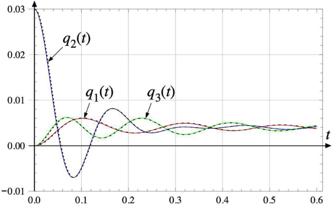

  

  Free vibration response obtained by using the general methodology. The response $q_1(t)$, $q_2(t)$, and $q_3(t)$ are indicated. Note that the initial conditions are satisfied

  Only the general treatment of analysis can be used to obtain the free vibration response. The response is plotted in Fig. 3. The free vibration response plotted in Fig. 3 has a steady-state deviation from zero (or the initial equilibrium position) for the amount of 0.004 m, the same as the rigid-body motion obtained in Eq. (43). The RB motion will cause the entire system to oscillate and asymptotically settles at a new position that is 0.004 m away from the initial equilibrium position. Thus, the free vibration response of such system resembles a “step response” based on the results shown in Fig. 3.

  We have also solved Eq. (38) using the same initial conditions with the numerical differential equation solver NDSolve[] of Mathematica, and overlaid the results by black dashed lines for each DoF in Fig. 3. Both solutions, one from the proposed analytical solution and the other from the numerical solver, are practically the same, which further validates the accuracy of the analytical methodology presented in this paper. The analytical solution, however, provides the physical insights of dynamic characteristics, as revealed in the damping ratios and natural frequencies in the modal space. For example, the low damping ratio, $\zeta$, associated with $\lambda _{1,2}$ in Table 2 is the main cause of the oscillatory response.

  Table 2 Damping ratios and natural frequencies of the 3 DoF unconstrained mechanical system

• ii. Forced vibration response: First, we determine the RB part of the forced vibration response. From Eq. (27), the RB part of the impulse response is

  $$\beta (t) = \mathcal{{L}}^{-1} \left\{ \frac{\mathbf{u }_0^T\mathbf{Q }}{s^2+(\mathbf{u }_0^T \mathbf{C u }_0)s} \right\} = 0.2582\, t$$

  where the impulse excitation is $\mathbf{Q }(t)=[\delta (t)\;0\;0]^T$. Note that $\mathbf{u }_0^T \mathbf{C u }_0=0$ in this example.

  Once the response $\beta (t)$ is found, the RB part of the forced vibration response can be determined by Eq. (20), $\mathbf{q }_{{RB}}(t) = \mathbf{u }_0\, \beta (t)$. Therefore, the RB part of the impulse is

  $$\mathbf{q }_{{RB}}(t) = \left[ \begin{array}{c} 0.06667 t \\ 0.06667 t \\ 0.06667 t \end{array} \right]$$

  (48)

  Next, let’s determine the NRB part of the forced vibration response.

  Employ the $\mathbf{A }$ matrix in Eq. (45) and the right/left eigenvectors in matrices $\mathbf{X }$ and $\mathbf{Y }$. The solution of the forced vibration response is given by the convolution integral in Eq. (31). The unit impulse response subject to $\mathbf{Q }(t)=[\delta (t)\;0\;0]^T$ is

  $$\begin{aligned} \mathbf{x }(t) &= \int _0^t \mathbf{X }\,e^{{\varvec{\Lambda }}(t-\tau )}\,\mathbf{Y }^T \,\mathbf{B }\,\mathbf{S }^T \mathbf{Q }(\tau )\,d\tau \\ &= \mathbf{X }\,e^{{\varvec{\Lambda }}t}\,\mathbf{Y }^T \,\mathbf{B }\,\mathbf{S }^T \left[ \begin{array}{c} 1 \\ 0 \\ 0 \end{array} \right] = \left[ \begin{array}{c} q^{\prime}_1 \\ q^{\prime}_2 \\ {\dot{q}}^{\prime}_1 \\ {\dot{q}}^{\prime}_2 \end{array} \right] \end{aligned}$$

  (49)

  The first two elements of $\mathbf{x }(t)$ are the reduced state vector $\mathbf{q^{\prime}}(t)$. Thus, the NRB part of the impulse response is $\mathbf{q }_{{{NRB}}}(t)=\mathbf{S\,q{^{\prime}}}(t)$

  $$\mathbf{q }_{{{NRB}}}(t) =\left[ \begin{array}{c} \mathbf{q }_{{{NRB},1}}\\ \mathbf{q }_{{{NRB},2}}\\ \mathbf{q }_{{{NRB},3}}\end{array}\right]$$

  (50)

  The overall response of forced vibration is the sum of the RB and NRB solutions obtained above. The impulse response is

  $$\mathbf{q }_{{imp}}(t)=\left[ \begin{array}{l} \mathbf{q }_{{imp,1}}\\ \mathbf{q }_{{imp,2}}\\ \mathbf{q }_{{imp,3}}\end{array} \right]$$

  (51)

  The details of the responses in Eqs. (49), (50) and (51) can be found in Appendix 2.

  The unit impulse response is plotted in Fig. 4.

  Fig. 4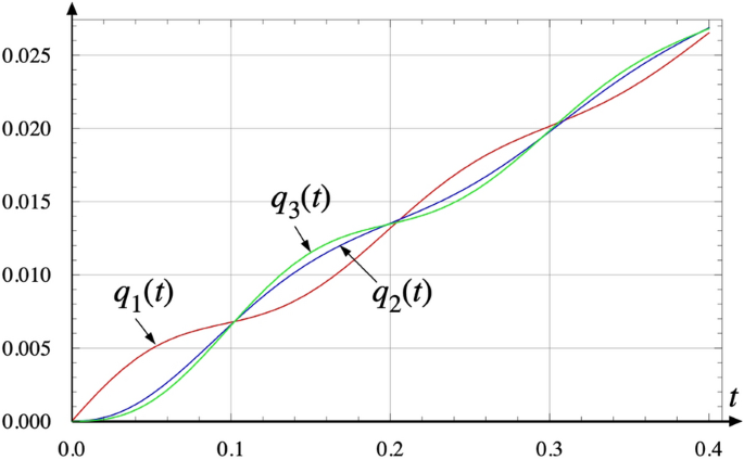

  

  Impulse response of the nonconservative system with damping. The response $q_1(t)$, $q_2(t)$, and $q_3(t)$ are indicated

  Note that the impulse response plotted in Fig. 4 is different from typical impulse responses of a constrained system. Due to the rigid-body motion, the entire system will continue to move away from the initial equilibrium position because of the RB motion in Eq. (48), which is a monotonically increasing motion, while the NRB oscillations are superposed on the RB motion. Thus, the impulse response of a unconstrained system resembles a ramp response of a constrained system.

Application of the theory to impedance control of redundant robots

The theory previously described and exemplified for vibration analysis of multi-DoF mechanical systems can be applied to obtain a closed-form solution of a multi-dimensional joint impedance control system of redundant and non-redundant robotic manipulators. A theoretically sound dynamic response of the robot can be obtained to modulate the behavior of the system through the choice of parameters of the stiffness and damping matrices.

Dynamic response of robotic manipulators performing Cartesian impedance control

In Cartesian impedance control, an n-DoF (redundant or non-redundant) robotic manipulator has a certain level of desired dynamic behavior when interacting with the environment [3]. The equations of motion of an n-DoF redundant manipulator is given by

$${\mathbf {M(q)}}{\ddot{\mathbf {q}}}(t)+{\mathbf {G}}{{(\mathbf q,{\dot{\mathbf q}})}}{\dot{\mathbf {q}}}(t)+{\mathbf {v(q)}}={\varvec{\tau }}_m+{\varvec{\tau }}_{ext}$$

(52)

where ${\mathbf {q}}$ is the vector of joint angles, M is the manipulator’s mass matrix, G the matrix containing the centrifugal and Coriolis terms and v is the gravity vector term. Choosing ${\varvec{\tau }}_m$ as $[-{\mathbf {K(q)q}}(t)-{\mathbf {C(q)}}{\dot{\mathbf {q}}}(t)+{\mathbf {v(q)}}+{\mathbf {G}{(\mathbf q,{\dot{\mathbf q}})}}{ {{\dot{\mathbf q}}}}(t)]$, the system in Eq. (52) becomes:

$${\mathbf {M(q)}}{\ddot{{\mathbf {q}}}}(t)+{\mathbf {C}}{\dot{\mathbf {q}}}(t)+{\mathbf {Kq}}(t)={\varvec{\tau }}_{ext}$$

(53)

This equation of impedance control is now comparable to Eq. (1) describing a mass, damper and spring system. In order to perform Cartesian impedance control, a desired dynamic behavior is intended in the Cartesian ($m \times m$) task space [7]

$${\mathbf {M}}_C{\ddot{\mathbf {x}}}(t)+{\mathbf {C}}_C{\dot{\mathbf {x}}}(t)+{\mathbf {K}}_C{\mathbf {x}}(t)={\mathbf {f}}$$

(54)

where, $\mathbf {K_C}$ is the Cartesian stiffness matrix, $\mathbf {C_C}$ is the damping matrix and $\mathbf {M_C}$ is the Cartesian mass matrix. The values of $\mathbf {K_C}$ can be chosen as necessary for the application, and a prospective initial damping matrix $\mathbf {C_C}$ can be approximated or based on relatively low values. Both Eqs. (53) and (54) assume the similar expression as that in Eq. (1); therefore, the preceding analysis can be employed to obtain dynamic response of impedance control. The impedance control in the joint space is often of primary interests because that is where the physical control is taking place with the motors and encoders. Thus, it is necessary to compute the respective stiffness, damping and mass matrices in the joint space with a specification of Cartesian task requirements.

For a given robot configuration, the inertia mass matrix $\mathbf{M }$ in the joint space can be computed [11], and the desired joint stiffness $\mathbf{K }$ and damping $\mathbf{C }$ matrices can be mapped from the Cartesian task space [5, 6, 12, 13] using the manipulator Jacobian $\mathbf{J }$:

$${\mathbf {K}}= {\mathbf {J}}^T{\mathbf {K}}_C{\mathbf {J}} + \mathbf{K }_G + \mathbf {J^TC}_C{\dot{\mathbf {J}}}$$

(55)

$${\mathbf {C}}= {\mathbf {J}}^T{\mathbf {C}}_C{\mathbf {J}}$$

(56)

where $\mathbf{K }_G = \left[ \left( \frac{\partial {\mathbf {J}}^T}{\partial q_1}{\mathbf {f}}\right) \left( \frac{\partial {\mathbf {J}}^T}{\partial q_2}{\mathbf {f}}\right) \cdots \left( \frac{\partial {\mathbf {J}}^T}{\partial q_n}{\mathbf {f}}\right) \right]$ is the equivalent stiffness due to the change of geometry under the presence of force [5].

Closed-form solution

Similar to the case of mechanical systems, we need to find a solution to Eq. (53) in the joint space. We assume that the external forces ${\mathbf {f}}$ and the changes in the Jacobian ${\mathbf {J}}$ of the manipulator are negligible, and only the first term in Eq. (55) is used to transform the stiffness matrix from Cartesian space to the joint space. With the stiffness and damping, $\mathbf{K }$ and $\mathbf{C }$ in Eqs. (55) and (56), used in Eq. (1), we can apply Eqs. (2) through (37) in the analysis of joint-space impedance control of robots, with a terminology change outlined in Table 3. The term of “zero-potential-energy,” or the ZP mode, is used in place of the RB motion, with identical physical meaning. The ZP motion will result in no net potential energy change from the stiffness matrix of the impedance control; that is, $\frac{1}{2}\,\mathbf{q }_{{{ZP}}}^T\mathbf{K }\,\mathbf{q }_{{{ZP}}}=0$, where $\mathbf{K }$ is the stiffness matrix of the impedance control in Eq. (53). Likewise, the NZP and NRB motions are also used with identical physical meaning.

Table 3 Comparison between discrete mechanical and robotic systems

This method accounts for the general case of possible redundant and non-redundant manipulators. In the former, this would be equivalent to the unconstrained systems, discussed earlier in the previous section. If the robotic manipulator system is non-redundant, it is no longer unconstrained, the dynamic response would only include the non-zero-potential-energy (NZP) part of the motion. Just like in the case for mechanical systems, the general dynamic response of the robot can be expressed as a linear combination of all the bases, ${\mathbf {u}}_i$, as in Eq. (6).

ZP and NZP motions

The ZP motion, represented by ${\mathbf {u}}_0$ in Eq. (2), can be determined and normalized, based on Eq. (20), as follows

$$\mathbf{q }_{{{ZP}}}(t)={\mathbf {u}}_0\beta (t)$$

(57)

where $\beta =\beta (t)$ is a function of time. Based on Eq. (21), we can substitute Eq. (57) into (53) to obtain

$${\mathbf {u}}_0^T\mathbf {Mu}_0{\ddot{\mathbf {\beta }}}(t) +{\mathbf {u}}_0^T\mathbf {Cu}_0{\dot{\mathbf {\beta }}}(t) = {\mathbf {u}}_0^T{\varvec{\tau }}_{ext}$$

(58)

Given that in general both K and C matrices go through similar transformations via the Jacobian matrix J, the second term in Eq. (58) will vanish. When ${\mathbf {u}}_0$ is normalized, this equation can be simplified as $\ddot{\mathbf {\beta }}(t)={\mathbf {u}}_0^T\mathbf {\tau _{ext}}$, and solved by including the initial conditions in this reduced space. To determine the oscillatory motions, we remove the known ZP mode ${\mathbf {q}}_i$ by imposing upon the state vector ${\mathbf {q}}$(t) a $n\! \times \! (n-1)$ constraint matrix, ${\mathbf {S}}$, as introduced earlier from Eq. (6) to Eq. (19), to build the ${\mathbf {M^{\prime}}}, {\mathbf {C}^{\prime}}$ and ${\mathbf {K^{\prime}}}$ matrices.

Once the NZP system is positive definite, we can obtain the NZP responses as described in the theory for mechanical discrete systems. After that, it is necessary to combine both ZP and NZP solutions, similar to Eq. (6) to finally obtain the full dynamic response. Then, a proper Cartesian damping matrix can be chosen [4]. Note that the complex conjugate eigenvalues render the natural frequency and damping ratio in the modal space, as follows

$$\lambda =a \pm i b; \quad \omega _d=b; \quad \zeta =cos(\gamma )$$

(59)

where a and b are the real and imaginary parts of the eigenvalues obtained in Eq. (31), and $\gamma =\tan ^{-1}(b/a)$. The dynamic response of the robotic system performing Cartesian or joint-based impedance control is determined by the damping ratios, $\zeta$, and the damped frequency, $\omega _d$, through a and b.

Special case of multiple redundancies

For cases when $r=n-m>1$, the methodology previously presented can also be applied; however, it is necessary to successively remove all r ZP modes from the system, while satisfying the orthogonality property with the mass matrix ${\mathbf {M}}$, as in Eq. (7), where each ${\mathbf {u}}_i$ represents a ZP mode.

With multiple redundancy and constraint matrices from the ZP modes, we have

$${\mathbf {q}} = \mathbf {Sq}^{r}={\mathbf {S}}_0 {\mathbf {S}}_1 \ldots {\mathbf {S}}_{r-1} {\mathbf {q}}^r$$

(60)

The r ZP modes of the system become an $(n \times r)$ matrix ${\mathbf {U}}_r$ containing the vectors of the null space of the stiffness matrix ${\mathbf {K}}$. There are two main ways of obtaining the NZP motions, as follows.

Successive removal of every ZP mode

Each ZP mode is removed one at a time, reducing the redundancy by one each time. This requires building a set of matrices using the constraint matrix each time until all r ZP modes are removed and the system becomes positive definite, as in the following.

$$\begin{aligned} \mathbf {Ku}_{0}&={\mathbf {0}}\rightarrow {\mathbf {q}}={\mathbf {S}}_0 {\mathbf {q^{\prime}}} \rightarrow {\mathbf {M^{\prime}}}, {\mathbf {C^{\prime}}}, {\mathbf {K^{\prime}}}\\ \mathbf {K^{\prime}u}_{0}^{\prime}&={\mathbf {0}}\rightarrow {\mathbf {q^{\prime}}}={\mathbf {S}}_1 {\mathbf {q^{\prime\prime}}} \rightarrow {\mathbf {M^{\prime\prime}}}, {\mathbf {C^{\prime\prime}}}, {\mathbf {K^{\prime\prime}}}\\ \mathbf {K^{\prime\prime}u}_{0^{\prime\prime}}&={\mathbf {0}}\rightarrow {\mathbf {q^{\prime\prime}}}={\mathbf {S}}_2 {\mathbf {q^{\prime\prime\prime}}} \rightarrow {\mathbf {M^{\prime\prime\prime}}}, {\mathbf {C^{\prime\prime\prime}}}, {\mathbf {K^{\prime\prime\prime}}}\\&\vdots& \\ {\mathbf {K}}^{r-1}{\mathbf {u}}^{r-1}_{0}&={\mathbf {0}}\rightarrow {\mathbf {q}}^{r-1}={\mathbf {S}}_{r-1} {\mathbf {q}}^{r} \rightarrow {\mathbf {M}}^{r}, {\mathbf {C}}^{r}, {\mathbf {K}}^{r} \end{aligned}$$

Abbreviated removal of ZP modes

Alternatively, all ZP modes can be removed by using the full ${\mathbf {U}}_r$ matrix to reduce the system directly into a $(n-r) \times (n-r)$ positive definite system. The following equations explain the procedures.

(61)

where ${\mathbf {u}}_1$ to ${\mathbf {u}}_{r-1}$ are derived with the following state variable transformations

$$\begin{aligned} {\mathbf {q}} & = {\mathbf {S}}_0 {\mathbf {q^{\prime}}}\rightarrow {\mathbf {q^{\prime}}}={\mathbf {S}}^*_0 {\mathbf {q}} \rightarrow {\mathbf {u}}_1^{\prime}={\mathbf {S}}^*_0 {\mathbf {u}}_1 \\ {\mathbf {q^{\prime}}}& = {\mathbf {S}}_1 {\mathbf {q^{\prime\prime}}}\rightarrow {\mathbf {q^{\prime\prime}}}={\mathbf {S}}^*_1 {\mathbf {q^{\prime}}} \rightarrow {\mathbf {u}}_2{^{\prime\prime}}={\mathbf {S}}^*_1 {\mathbf {S}}^*_0 {\mathbf {u}}_2\\ & \vdots & \\ {\mathbf {q}}^{r-2} &= {\mathbf {S}}_{r-2} {\mathbf {q}}^{r-1}\rightarrow {\mathbf {q}}^{r-1}={\mathbf {S}}^*_{r-2} {\mathbf {q}}^{r-2} \\ \rightarrow {\mathbf {u}}_{r-1}^{r-1}& ={\mathbf {S}}^*_{r-2} {\mathbf {S}}^*_{r-3} \ldots {\mathbf {S}}^*_0 {\mathbf {u}}_{r-1} \\ {\mathbf {q}}^{r-1} & = {\mathbf {S}}_{r-1}{\mathbf {q}}^{r}\rightarrow {\mathbf {M}}^{r}, {\mathbf {C}}^{r}, {\mathbf {K}}^{r} \end{aligned}$$

Both ways of removing ZP modes are further explained in the following example of robotic impedance control.

Example of a redundant 7-DoF robot

The example used to illustrate the analysis is a general robotic system which consists of 7 DoF. We choose to consider a Cartesian impedance control with 5 DoF to demonstrate the procedures to handle multiple redundancy. Therefore, we have $n=7$ and $m=5$ in this case, giving two-DoF redundancy with $r=2$. Both methods of successive removal of the ZP modes in (i) and the abbreviated method in (ii) are employed.

At a chosen robotic configuration, there is a Jacobian matrix ${\mathbf {J}}$ associated with it, as well as a mass matrix ${\mathbf {M}}$, and a chosen set of stiffness and damping matrices ${\mathbf {K}}$ and ${\mathbf {C}}$ mapped from the Cartesian space. All these matrices can be found in Appendix 3, at the end of the paper. The $7 \times 7$ impedance control equation in the joint space is

$$\mathbf{M }\,{\ddot{\mathbf{q }}}(t) + \mathbf{C }\,{\dot{\mathbf{q }}}(t) + \mathbf{K }\,\mathbf{q }(t) = \mathbf{Q }$$

where the mass, damping and stiffness matrices are:

$$\begin{aligned} {\mathbf {M}} &= \left[ \begin{array}{cccc} 3.414 & -0.6947 & -0.1556 & -0.4560 \\ -0.6947 & 8.710 & 0.3832 & 5.484 \\ -0.1556 & 0.3832 & 3.860 & 0.1785 \\ -0.4560 & 5.484 & 0.1785 & 4.831 \\ 1.934 & 0.1270 & 1.995 & 0.04439 \\ -0.3131 & 3.108 & 0.2056 & 2.444 \\ 0.2101 & -0.08658 & 0.1165 & -0.07011 \end{array} \right. \\&\left. \begin{array}{ccc} 1.934 & -0.3131 & 0.2101 \\ 0.1270 & 3.108 & -0.08658 \\ 1.995 & 0.2056 & 0.1165 \\ 0.04439 & 2.444 & -0.07011 \\ 2.770 & -0.01395 & 0.2296 \\ -0.01395 & 2.459 & -0.07805 \\ 0.2296 & -0.07805 & 0.08852 \end{array} \right] \\ {\mathbf {C}} &= \left[ \begin{array}{cccc} 1.949 & 0.07297 & 1.305 & 0.1258 \\ 0.07297 & 2.956 & -0.3774 & 2.388 \\ 1.305 & -0.3774 & 1.963 & -0.3420 \\ 0.1258 & 2.388 & -0.3420 & 2.173 \\ 0.5526 & -0.4693 & 1.623 & -0.4543 \\ 0.09194 & 1.670 & -0.3647 & 1.738 \\ 0 & -0.05528 & 0.1413 & -0.05528 \end{array}\right. \\&\left. \begin{array}{ccc} 0.5526 & 0.09194 & 0 \\ -0.4693 & 1.670 & -0.05528 \\ 1.623 & -0.3647 & 0.1413 \\ -0.4543 & 1.738 & -0.05528 \\ 1.597 & -0.4639 & 0.1625 \\ -0.4639 & 1.657 & -0.05528 \\ 0.1625 & -0.05528 & 0.01833 \end{array} \right] \\ {\mathbf {K}} & = \left[ \begin{array}{cccc} 162.4 & 7.297 & 108.7 & 12.58 \\ 7.297 & 71.02 & 3.605 & 51.40 \\ 108.7 & 3.605 & 78.97 & 7.147 \\ 12.58 & 51.40 & 7.147 & 48.11 \\ 46.05 & 0.5985 & 37.93 & 2.098 \\ 9.194 & 20.69 & 4.876 & 27.30 \\ 0 & -0.1658 & 0.8012 & -0.1658 \end{array}\right. \\&\left. \begin{array}{ccc} 46.05 & 9.194 & 0 \\ 0.5985 & 20.69 & -0.1658 \\ 37.93 & 4.876 & 0.8012 \\ 2.098 & 27.30 & -0.1658 \\ 21.22 & 1.136 & 0.9211 \\ 1.136 & 21.57 & -0.1658 \\ 0.9211 & -0.1658 & 0.1039 \end{array}\right] \end{aligned}$$

As stated in the theory, the characteristic of an unconstrained, positive semi-definite system is a singular stiffness matrix, $\mathbf{K }$. For this case, the eigenvalues of the stiffness matrix are:

$$eig({\mathbf {K}}) = \left[ 255.1, 120.8, 16.85, 10.03, 0.5840, 0, 0 \right]$$

This system is not solvable, unless the two ZP modes (r = 2) are removed. Once this is done, we can solve for the oscillatory and non-oscillatory motions as presented in Eqs. (2)–(37).

Successive removal of every ZP mode

The stiffness matrix ${\mathbf {K}}$ is associated with two ZP modes. Both ZP modes belong to the null space of ${\mathbf {K}}$. When normalized and making them orthogonal to each other, we obtain

(62)

In order to remove the first ZP mode we use the first vector ${\mathbf {u}}_0$ to build its corresponding constraint matrix ${\mathbf {S}}_0$, such that

$$\begin{aligned}{\mathbf {q}}&= [{\mathbf {q}}_1\, {\mathbf {q}}_2\, {\mathbf {q}}_3\, {\mathbf {q}}_4\, {\mathbf {q}}_5\, {\mathbf {q}}_6\, {\mathbf {q}}_7]^T = {\mathbf {S}}_0 \, {\mathbf {q^{\prime}}} \\&= \left[ \begin{array}{cccccc} 1 & 0 & 0 & 0 & 0 & 0\\ 0 & 1 & 0 & 0 & 0 & 0\\ 0 & 0 & 1 & 0 & 0 & 0\\ 0 & 0 & 0 & 1 & 0 & 0\\ 0 & 0 & 0 & 0 & 1 & 0\\ 0 & 0 & 0 & 0 & 0 & 1\\ -17.0 & 3.12 & 11.5 & 1.86 & -6.3 & 1.94\\ \end{array}\right] \left[ \begin{array}{c} {\mathbf {q}}_1\\ {\mathbf {q}}_2\\ {\mathbf {q}}_3\\ {\mathbf {q}}_4\\ {\mathbf {q}}_5\\ {\mathbf {q}}_6 \end{array}\right] \\ \end{aligned}$$

With this constraint matrix ${\mathbf {S}}_0$ we can now build a new system free of this first ZP mode:

$${\mathbf {M^{\prime}}} ={\mathbf {S}}_0^T {\mathbf {M}} {\mathbf {S}}_0;\; {\mathbf {C^{\prime}}} ={\mathbf {S}}_0^T {\mathbf {C}} {\mathbf {S}}_0;\; {\mathbf {K^{\prime}}} ={\mathbf {S}}_0^T {\mathbf {K}} {\mathbf {S}}_0$$

The numerical values for these matrices are in Appendix 3. This $6 \times 6$ system in the reduced space ${\mathbf {q^{\prime}}}$ is still not free from the second ZP mode ${\mathbf {u}}_1$. The system is not positive definite, with the eigenvalues of

$$eig({\mathbf {K^{\prime}}}) = \left[ 252.55, 120.22, 67.585, 16.587, 0.5843, 0 \right]$$

In order to remove the remaining ZP mode, we need to build a second constraint matrix ${\mathbf {S}}_1$ by first obtaining and normalizing this ZP mode from ${\mathbf {K^{\prime}}}$ in the next reduced space of ${\mathbf {K^{\prime}}} {\mathbf {u^{\prime}}}_1={\mathbf {0}}$ and ${\mathbf {S}}_0 \, {\mathbf {u^{\prime}}}_1= {\mathbf {u}}_1$. Once this ZP mode is obtained we can build ${\mathbf {S}}_1$ with

$$\begin{aligned} {\mathbf {q^{\prime}}}&= [{\mathbf {q^{\prime}}}_1\, {\mathbf {q^{\prime}}}_2\, {\mathbf {q^{\prime}}}_3\, {\mathbf {q^{\prime}}}_4\, {\mathbf {q^{\prime}}}_5\, {\mathbf {q^{\prime}}}_6]^T \\ &= \left[ \begin{array}{ccccc} 1 & 0 & 0 & 0 & 0\\ 0 & 1 & 0 & 0 & 0\\ 0 & 0 & 1 & 0 & 0\\ 0 & 0 & 0 & 1 & 0\\ 0 & 0 & 0 & 0 & 1\\ 22.4 & -1.93 & -14.1 & -0.813 & 9.48 \\ \end{array}\right] \left[ \begin{array}{c} {\mathbf {q^{\prime}}}_1\\ {\mathbf {q^{\prime}}}_2\\ {\mathbf {q^{\prime}}}_3\\ {\mathbf {q^{\prime}}}_4\\ {\mathbf {q^{\prime}}}_5\\ \end{array}\right] \nonumber \\ &= {\mathbf {S}}_1 \, {\mathbf {q^{\prime\prime}}} \end{aligned}$$

(63)

With this constraint matrix ${\mathbf {S}}_1$ the new system in the ${\mathbf {q^{\prime\prime}}}$ space can be found

$${\mathbf {M^{\prime\prime}}} = {\mathbf {S}}_1^T {\mathbf {M^{\prime}}} {\mathbf {S}}_1;\; {\mathbf {C^{\prime\prime}}} ={\mathbf {S}}_1^T {\mathbf {C^{\prime\prime}}} {\mathbf {S}}_1;\; {\mathbf {K^{\prime\prime}}} ={\mathbf {S}}_1^T {\mathbf {K^{\prime}}} {\mathbf {S}}_1$$

The numerical values of these matrices are in Appendix 3. Now, this system is positive definite since both ZP modes have been removed, with the eigenvalues of

$$eig({\mathbf {K^{\prime\prime}}}) = \left[ 17186, 197.01, 63.79, 10.023, 0.8841 \right]$$

This ($5\!\times \!5$) system is now solvable by applying the theory of mechanical vibration of discrete systems presented ealier.

Next, we are going to show that the abbreviated method is equivalent to removing the ZP modes successively one at a time.

Alternative method to remove ZP modes

From Eqs. (61) and (62) and information of every ZP mode, we can build the constraint matrices. For ${\mathbf {S}}_0$, we can directly use ${\mathbf {u}}_0$

$$\begin{aligned} {\mathbf {q}} &= [{\mathbf {q}}_1\, {\mathbf {q}}_2\, {\mathbf {q}}_3\, {\mathbf {q}}_4\, {\mathbf {q}}_5\, {\mathbf {q}}_6\, {\mathbf {q}}_7]^T = {\mathbf {S}}_0 \, {\mathbf {q^{\prime}}} \\ &= \left[ \begin{array}{cccccc} 1 & 0 & 0 & 0 & 0 & 0\\ 0 & 1 & 0 & 0 & 0 & 0\\ 0 & 0 & 1 & 0 & 0 & 0\\ 0 & 0 & 0 & 1 & 0 & 0\\ 0 & 0 & 0 & 0 & 1 & 0\\ 0 & 0 & 0 & 0 & 0 & 1\\ -17.04 & 3.118 & 11.45 & 1.86 & -6.304 & 1.94 \end{array}\right] \left[ \begin{array}{c} {\mathbf {q}}_1\\ {\mathbf {q}}_2\\ {\mathbf {q}}_3\\ {\mathbf {q}}_4\\ {\mathbf {q}}_5\\ {\mathbf {q}}_6\\ \end{array}\right] \end{aligned}$$

We can now use ${\mathbf {S}}_0$ to obtain the next ZP mode in the reduced space ${\mathbf {q^{\prime}}}$ with ${\mathbf {u^{\prime}}}_1={\mathbf {S}}_0^*\,{\mathbf {u}}_1$, where ${\mathbf {S}}_0^*$ is the pseudo-inverse of the first constraint matrix, and ${\mathbf {u}}_1$ is the next ZP mode in the original ($7\times 7$) space. It is important to always work with the ZP vectors normalized with respect to ${\mathbf {M}}$, and the inverse of ${\mathbf {S}}_0$ must be unique and consistent with ${\mathbf {M}}$, i.e. ${\mathbf {S}}_0^*=({\mathbf {S}}_0^T{\mathbf {M}}{\mathbf {S}}_0)^{-1}{\mathbf {S}}_0^T{\mathbf {M}}$. Once this ($6 \times 1$) ZP mode, $\mathbf{u }_1^{\prime}$, is obtained, the ${\mathbf {S}}_1$ constraint matrix, with ${\mathbf {q^{\prime}}}={\mathbf {S}}_1 \, {\mathbf {q^{\prime\prime}}}$, can be constructed as follows

$${\mathbf {q^{\prime}}} = \left[ \begin{array}{ccccc} 1 & 0 & 0 & 0 & 0\\ 0 & 1 & 0 & 0 & 0\\ 0 & 0 & 1 & 0 & 0\\ 0 & 0 & 0 & 1 & 0\\ 0 & 0 & 0 & 0 & 1\\ 22.4 & -1.93 & -14.1 & -0.813 & 9.48\\ \end{array}\right] \left[ \begin{array}{c} {\mathbf {q^{\prime\prime}}}_1\\ {\mathbf {q^{\prime\prime}}}_2\\ {\mathbf {q^{\prime\prime}}}_3\\ {\mathbf {q^{\prime\prime}}}_4\\ {\mathbf {q^{\prime\prime}}}_5\\ \end{array}\right]$$

This is exactly the same as the $\mathbf{S }_1$ obtained in Eq. (63) from successive removal of the ZP modes. The full constraint matrix ${\mathbf {S}}$ can be obtained without needing to build systems in each step, and as in Eq. (60)

$$\mathbf{q }_{{{NZP}}}= \mathbf {S\,q^{\prime\prime}}={\mathbf {S}}_0 {\mathbf {S}}_1\, {\mathbf {q^{\prime\prime}}}$$

With $\mathbf{S }={\mathbf {S}}_0 {\mathbf {S}}_1$, the matrix can be written as

$${\mathbf {S}} = \left[ \begin{array}{ccccc} 1 & 0 & 0 & 0 & 0\\ 0 & 1 & 0 & 0 & 0\\ 0 & 0 & 1 & 0 & 0\\ 0 & 0 & 0 & 1 & 0\\ 0 & 0 & 0 & 0 & 1\\ 22.36 & -1.925 & -14.08 & -0.8126 & 9.478\\ 26.43 & -0.6264 & -15.93 & 0.2800 & 12.12\\ \end{array}\right]$$

With this full constraint matrix ${\mathbf {S}}$, we can obtain the positive definite system directly as follows

$${\mathbf {M^{\prime\prime}}} = {\mathbf {S}}^T {\mathbf {M}} {\mathbf {S}};\; {\mathbf {C^{\prime\prime}}} = {\mathbf {S}}^T {\mathbf {C}} {\mathbf {S}}; \; {\mathbf {K^{\prime\prime}}} = {\mathbf {S}}^T {\mathbf {K}} {\mathbf {S}}$$

The results are identical to the system obtained by using the method of building a new system by successively removing each ZP presented earlier. This reduced system leads to the following damping ratios and natural frequencies. It is noted that there are 3 modes with small damping ratios, $\zeta$, in Table 4.

Table 4 Damping ratios and natural frequencies of the Baxter robot performing Cartesian impedance control for a given set of damping and stiffness matrices

Solve the positive definite system

This positive definite system $\{\mathbf{M^{\prime\prime}}, \mathbf{C^{\prime\prime}}, \mathbf{K^{\prime\prime}}\}$ now can be solved by using Eqs. (29) to (32) of the dual eigenvalue analysis. An initial displacement of the following is given to the system

$${\mathbf {q}}(0)=[ \begin{array}{ccccccc} 0&0.01&0.01&0&0&0&0 \end{array}]^T rad$$

The response of NZP motion $q_1^{\prime\prime}$ to $q_5^{\prime\prime}$ denoted by

$${\mathbf {q^{\prime\prime}}}(t) =[q_1^{\prime\prime}(t)\, q_2^{\prime\prime}(t)\, q_3^{\prime\prime}(t)\, q_4^{\prime\prime}(t)\, q_5^{\prime\prime}(t)]^T$$

can be obtained by following the methodology of the dual eigenvector analysis. The results of $q_1^{\prime\prime}$ to $q_5^{\prime\prime}$ are in Appendix 3.

The dynamic response of the physical system $\mathbf{q }(t)$ can now be obtained by the following equation

$$\mathbf{q }(t) = \mathbf{q }_{{{ZP}}}+ \mathbf{S }_0\, \mathbf{S }_1 {\mathbf {q^{\prime\prime}}}(t)$$

(64)

where the NZP component from Eq. (37) is $\mathbf{q }_{{{NZP}}}= \mathbf{S }_0\, \mathbf{S }_1 {\mathbf {q^{\prime\prime}}}(t)$. The results are plotted in Fig. 5 where both ZP and NZP parts of the response are combined in the responses from $q_1$ to $q_7$.

Fig. 5

Free vibration response obtained by using the general methodology, showing the characteristics of dynamic response of this system. Note that the initial conditions are satisfied

The dynamic response in Fig. 5 is plotted for the first five seconds to illustrate the characteristics of free vibration response. The results are indicative of the typical behavior and can give a glimpse of the characteristics of dynamic response of the impedance control through the overshoots and settling times of the response. When plotted over a longer period of time, we can examine the low damping characteristics with low frequency that takes longer to settle.

Discussion

Free vibration responses of a unconstrained and non-conservative discrete mechanical system with prescribed initial displacement show that the responses resemble a step response of a system with external force, due primarily to the RB mode of the unconstrained system. As shown in the plots of the combined RB and NRB motions, the initial conditions are satisfied. Likewise, an impulse response of a unconstrained mechanical system has a forced vibration response that resembles a ramp response of forced vibration, due to the RB mode.

It is noted that the coefficient of the $\ddot{\beta }$ term in Eq. (23) will not be unity unless the RB mode, $\mathbf{u }_0$, is normalized with respect to the mass matrix, as defined in Eq. (7). In the case of free vibration, when $\mathbf{u }_0$ is not normalized according to Eq. (7), the non-unity coefficient will disappear from the homogenous equation and can result in incorrect RB component of the initial condition. On the other hand, forced vibration in Eq. (22) will not be affected because the coefficient will be carried through with the non-zero forcing function term $\mathbf{u }_0^T\mathbf{Q }$.

In applying the methodology to an example of impedance control of a Baxter robot, the complex eigenvalues of the $5\! \times \! 5$ positive definite system in the reduced space of robotic impedance control are $-1.450 \pm i14.54$, $-0.3116 \pm i3.700$, $-0.1833 \pm i3.066$, $-0.3660 \pm i2.046$ and $-0.04169 \pm i0.8158$. These complex eigenvalues result in damping ratios, $\zeta$, and natural frequencies, $\omega _n$ listed in Table 4. It is noted that the damping ratios are low, resulting in highly oscillatory responses, as shown in the responses plotted in Fig. 5. Since the responses of $q_1$ to $q_7$ are the linear combination of the bases obtained from the $5\!\times \! 5$ positive definite system, the lower damping ratios, especially when accompanied by low natural frequency, will appear in $q_1$ to $q_7$ to dominate the response. It is important to be able to increase the damping ratios in order to improve the overall dynamic responses.

This can be achieved, with a given stiffness matrix, by choosing different values in the elements of damping matrix. However, study shows that increasing all elements of the damping matrix may not necessarily improve all damping ratios. Furthermore, certain elements of the damping matrix have more influence on certain damping ratios of the complex eigenvalues. The methodology presented in this paper, nevertheless, can assist in determining which diagonal and/or off-diagonal elements in the damping matrix can improve the damping ratios. This reduces blind guessing or trial-and-error in choosing values of the elements of the damping matrix [4, 6] to improve dynamic response.

By applying the dual eigenvalue analysis in Eqs. (29) to (32), we are able to evaluate the dynamic response of the impedance control by criteria such as damping ratios and frequency of the NZP part of the motion. This methodology with the closed-form solution allows us to adjust the stiffness and damping parameters in the ${\mathbf {K}}$ and ${\mathbf {C}}$ matrices, respectively, according to the required applications of the performance of dynamic responses. It also allows us to modulate the dynamic response of the null space of the robotic task [14,15,16]. If there are any desired additional tasks for the redundant DoF(s), the stiffness and damping parameters can be mapped into the joint space by the use of a null space projection matrix, and from there on, proceed as shown here. In summary, the methodology presented in this paper can provide the advantage to systematically adjust the elements in $\mathbf{K }$ and $\mathbf{C }$ matrices of impedance control to modulate the dynamic responses of the system.

As a case in point, when trying to perform impedance control in the Cartesian ($6 \times 6$) space using a redundant 7-DoF manipulator at a chosen configuration, the given stiffness for the task is

$${\mathbf {K}}_C=diag([3000, 3000, 3000, 100, 100, 100])$$

An initial damping matrix is picked as

$${\mathbf {C}}_{C0}={\mathbf {I}}_6$$

The following damping ratios can be obtained: 0.0108, 0.0039, 0.0162, 0.0342, 0.116 and 0.0953. In contrast, if we apply the methodology presented here to select a damping matrix, one possible non-diagnoal damping matrix, after a synthesis using the methodology, is

$${\mathbf {C}}_{C1}=\left[ \begin{array}{cccccc} 0.1 & 0 & 0 & 0 & 0 & 0\\ 0 & 0.1 & 0 & 0 & 0 & 0\\ 0 & 0 & 0.1 & 0 & 10 & 0\\ 0 & 0 & 0 & 10 & 0 & 0\\ 0 & 0 & 10 & 0 & 10 & 0\\ 0 & 0 & 0 & 0 & 0 & 1 \end{array}\right]$$

The damping ratios of ${\mathbf {C}}_{C1}$ are: 0.0326, 0.1081, 0.1335, 0.3419, 0.1342 and 0.1274. This revised impedance control with the new ${\mathbf {C}}_{C1}$ damping matrix has a better dynamic response because of the improvement of damping ratios of the multiple DoF system.

Conclusion

A general methodology to obtain a closed-form solution for free and forced vibration responses are presented for unconstrained mechanical system and robotic manipulators under impedance control. The methodology includes a novel procedure to deal with nonconservative unconstrained systems or redundant robots containing rigid body (RB) or zero potential energy (ZP) modes, which must be removed, using constraint matrix, to obtain the dynamic response. After that, the non-positive definite system can be mapped via constraint matrix to form a positive definite system in a reduced space, to obtain the complete dynamic response of the system.

When applying to robotic manipulators performing Cartesian and joint-based impedance control, this methodology can provide the analysis and synthesis of dynamic characteristics of the impedance control system. This theory can help in choosing the elements of the damping matrix to attain prescribed dynamic response with damping characteristics without guessing or trial-and-error. The elimination of trial-and-error in determining the elements of the damping matrix in impedance control to meet the requirements of dynamic response, by using this novel analytical methodology, is another important contribution of this paper. The methodology was illustrated by examples of both a discrete mechanical system and a redundant robotic manipulator in impedance control with damping modulation.

Appendices

Appendix 1: Results in the example of free vibration

The results of $\mathbf{q }_{{{NRB}}}(t)$ in Eq. (46) are: $\begin{aligned}\mathbf{q }_{NRB,1} & = e^{-3.024t}(-0.002293\,\cos 30.83\,t -0.001256\,\sin 30.83\,t)\\ & \quad +e^{-10.29t}(-0.001707\,\cos 38.88\,t+0.0003660\,\sin 38.88\,t), \end{aligned}$

$\begin{aligned} \mathbf{q }_{{NRB},2} &= e^{-3.024t}(0.001563\,\cos 30.83\,t +0.001344\,\sin 30.83\,t)\\ & \quad +e^{-10.29t}(0.02444\,\cos 38.88\,t+0.005522\,\sin 38.88\,t), \end{aligned}$ and

$$\begin{aligned} \mathbf{q }_{{NRB},3} &= e^{-3.024t}(0.003044\,\cos 30.83\,t +0.001472\,\sin 30.83\,t) \\ & \quad +e^{-10.29t}(-0.007044\,\cos 38.88\,t-0.002794\,\sin 38.88\,t). \end{aligned}$$

The results of q(t) in Eq. (47) are: $\begin{aligned} q_1(t) & = 0.004 +e^{-3.024t}(-0.002293\,\cos 30.83\,t-0.001256\,\sin 30.83\,t) \\ & \quad +e^{-10.29t}(-0.001707\,\cos 38.88\,t+0.0003660\,\sin 38.88\,t), \end{aligned}$

$\begin{aligned} q_2(t)& = 0.004 +e^{-3.024t}(0.001563\,\cos 30.83\,t +0.001344\,\sin 30.83\,t) \\ & \quad +e^{-10.29t}(0.02444\,\cos 38.88\,t+0.005522\,\sin 38.88\,t), \end{aligned}$ and

$$\begin{aligned} q_3(t) &= 0.004 +e^{-3.024t}(0.003044\,\cos 30.83\,t +0.001472\,\sin 30.83\,t)\\ & \quad +e^{-10.29t}(-0.007044\,\cos 38.88\,t-0.002794\,\sin 38.88\,t). \end{aligned}$$

Appendix 2: Results in the example of forced vibration

The results of $q^{\prime}_1$ to $q^{\prime}_4$ in Eq. (49) are: $q^{\prime}_1= e^{-3.024t}(-0.00004006\,\cos 30.83t +0.001863\sin 30.83t) +e^{-10.29t}(0.00004006\,\cos 38.88t+0.00003087\sin 38.88t),$

$$\begin{aligned} q^{\prime}_2 &= e^{-3.024t}(0.0003357\,\cos 30.83t-0.001430\sin 30.83t) \\ & \quad +e^{-10.29t}(-0.0003357\,\cos 38.88t-0.0006435\sin 38.88t), \end{aligned}$$

$\begin{aligned} {\dot{q}}^{\prime}_1& = e^{-3.024t}(0.05755\,\cos 30.83t-0.004398\sin 30.83t) \\ & \quad +e^{-10.29t}(0.0007881\,\cos 38.88t-0.001875\sin 38.88t)\end{aligned}$ and

$$\begin{aligned} {\dot{q}}^{\prime}_2& = e^{-3.024t}(-0.04510\,\cos 30.83t-0.006025\sin 30.83t) \\ & \quad +e^{-10.29t}(-0.02157\,\cos 38.88t+0.01967\sin 38.88t). \end{aligned}$$

The results of $\mathbf{q }_{{{NRB}}}$ in Eq. (50) are: $\begin{aligned} \mathbf{q }_{{NRB},1} &= e^{-3.024t}(-0.00004006\,\cos 30.83t+0.001863\sin 30.83t) \\ & \quad +e^{-10.29t}(0.00004006\,\cos 38.88t+0.00003087\sin 38.88t), \end{aligned}$

$\begin{aligned} \mathbf{q }_{{NRB},2}& = e^{-3.024t}(0.0003357\,\cos 30.83t -0.001430\sin 30.83t) \\ & \quad +e^{-10.29t}(-0.0003357\,\cos 38.88t-0.0006435\sin 38.88t)\end{aligned}$ and

$$\begin{aligned} \mathbf{q }_{{{NRB},3}} & = e^{-3.024t}(-0.00007018\,\cos 30.83t -0.002408\sin 30.83t) \\ & \quad +e^{-10.29t}(0.00007018\,\cos 38.88t+0.0002080\sin 38.88t). \end{aligned}$$

The results of $\mathbf{q }(t)$ in Eq. (51) are: $\begin{aligned} \mathbf{q }_{imp,1} & = 0.06667t +e^{-3.024t}(-0.00004006\,\cos 30.83t +0.001863\sin 30.83t) \\ & \quad +e^{-10.29t}(0.00004006\,\cos 38.88t+0.00003087\sin 38.88t), \end{aligned}$

$\begin{aligned} \mathbf{q }_{imp,2}& = 0.06667t+e^{-3.024t}(0.0003357\,\cos 30.83t-0.001430\sin 30.83t) \\ & \quad +e^{-10.29t}(-0.0003357\,\cos 38.88t-0.0006435\sin 38.88t), \end{aligned}$ and

$$\begin{aligned} \mathbf{q }_{imp,3}& = 0.06667t+e^{-3.024t}(-0.00007018\,\cos 30.83t-0.002408\sin 30.83t)\\ & \quad +e^{-10.29t}(0.00007018\,\cos 38.88t+0.0002080\sin 38.88t).\end{aligned}$$

Appendix 3: Matrices and results from the example of impedance control

The matrices for the robotic impedance control application example are:

$$\begin{aligned} {\mathbf {J}}(\mathbf{q} ) &= \left[ \begin{array}{cccc} -0.57 & -0.1280 & -0.3816 & -0.2208 \\ 0.57 & -0.1280 & 0.3816 & -0.2208 \\ 0 & -0.7371 & 0 & -0.3903 \\ 0 & -0.7071 & 0.6028 & -0.7071 \\ 0 & 0.7071 & 0.6028 & 0.7071 \end{array} \right. \\& \left. \begin{array}{ccc} -0.1616 & -0.1613 & 0 \\ 0.1616 & -0.1613 & 0 \\ 0 & -0.02537 & 0 \\ 0.6930 & -0.7071 & 0.07818 \\ 0.6930 & 0.7071 & 0.07818 \end{array} \right] \\ {\mathbf {K}}_C &= diag([300, 200, 100, 10, 7])\\ {\mathbf {C}}_C &= diag([3.5, 2.5, 2.5, 2, 1]) \end{aligned}$$

The matrices in the first reduced space for the robotics example are:

$$\begin{aligned} {\mathbf {M^{\prime}}}& = {\mathbf {S}}_0^T {\mathbf {M}} {\mathbf {S}}_0\\& = \mathbf { \left[ \begin{array}{cccccc} 21.97 & -3.269 & -17.02 & -1.677 & 6.208 & -1.508\\ -3.269 & 9.030 & 2.916 & 5.617 & -0.3513 & 3.232\\ -17.02 & 2.916 & 18.14 & 1.478 & -2.502 & 1.509\\ -1.677 & 5.617 & 1.478 & 4.876 & -0.1245 & 2.482\\ 6.208 & -0.3513 & -2.502 & -0.1245 & 3.393 & -0.1605\\ -1.508 & 3.232 & 1.509 & 2.482 & -0.1605 & 2.490 \end{array}\right] }\\ {\mathbf {C^{\prime}}} & = {\mathbf {S}}_0^T {\mathbf {C}} {\mathbf {S}}_0\\ &= \mathbf { \left[ \begin{array}{cccccc} 7.278 & 0.04066 & -4.6863 & 0.4868 & -0.2475 & 0.4265\\ 0.04066 & 2.790 & 0.08515 & 2.219 & 0.02553 & 1.501\\ -4.686 & 0.08515 & 7.609 & -0.3215 & 1.269 & -0.3146\\ 0.4868 & 2.219 & -0.3215 & 2.031 & -0.0185 & 1.594\\ -0.2475 & 0.02553 & 1.269 & -0.0185 & 0.2768 & -0.0241\\ 0.4265 & 1.501 & -0.3146 & 1.594 & -0.0241 & 1.512\\ \end{array}\right] }\\ {\mathbf {K^{\prime}}} & = {\mathbf {S}}_0^T {\mathbf {K}} {\mathbf {S}}_0\\ & = \mathbf { \left[ \begin{array}{cccccc} 192.6 & 4.599 & 74.80 & 12.11 & 41.52 & 8.577\\ 4.599 & 70.99 & 7.915 & 51.17 & 2.473 & 20.48\\ 74.80 & 7.915 & 110.9 & 8.951 & 35.93 & 6.848\\ 12.11 & 51.17 & 8.951 & 47.85 & 3.638 & 27.04\\ 41.52 & 2.473 & 35.93 & 3.638 & 13.73 & 2.699\\ 8.577 & 20.48 & 6.848 & 27.04 & 2.699 & 21.32\\ \end{array}\right] } \end{aligned}$$

The matrices in the second (positive definite) reduced space for the robotics example are:

$$\begin{aligned} {\mathbf {M^{\prime\prime}}} &= {\mathbf {S}}_1^T {\mathbf {M^{\prime}}} {\mathbf {S}}_1 = {\mathbf {S}}^T {\mathbf {M}} {\mathbf {S}}\\ &= \mathbf { \left[ \begin{array}{ccccc} 1200 & -35.30 & -746.4 & 9.815 & 516.2\\ -35.30 & 5.813 & 22.01 & 2.106 & -14.85\\ -746.4 & 22.01 & 469.6 & -6.214 & -318.4\\ 9.815 & 2.106 & -6.214 & 2.485 & 4.357\\ 516.2 & -14.85 & -318.4 & 4.357 & 224.08 \end{array}\right] }\\ {\mathbf {C^{\prime\prime}}} &= {\mathbf {S}}_1^T {\mathbf {C^{\prime}}} {\mathbf {S}}_1={\mathbf {S}}^T {\mathbf {C}} {\mathbf {S}}\\ &= \mathbf { \left[ \begin{array}{ccccc} 782.6 & -32.31 & -494.04 & 8.318 & 323.7\\ -32.31 & 2.612 & 20.55 & 0.2951 & -13.29\\ -494.04& 20.55 & 316.4 & -5.216 & -203.2\\ 8.318 & 0.2951 & -5.216 & 0.4382 & 3.467\\ 323.7 & -13.29 & -203.2 & 3.467 & 135.6 \end{array}\right] }\\ {\mathbf {K^{\prime\prime}}}& = {\mathbf {S}}_1^T {\mathbf {K^{\prime}}} {\mathbf {S}}_1 = {\mathbf {S}}^T {\mathbf {K}} {\mathbf {S}}\\ &= \mathbf { \left[ \begin{array}{ccccc} 11240.5 & -472.08 & -6609.2 & 222.44 & 4703\\ -472.08 & 71.17 & 284.5 & 15.82 & -197.7\\ -6609.2 & 284.5 & 4148.1 & -133.4 & -2783.8\\ 222.44 & 15.82 & -133.4 & 17.98 & 93.54\\ 4703 & -197.7 & -2783.8 & 93.54 & 1980.5 \end{array}\right] } \end{aligned}$$

The individual results from $q_1^{\prime\prime}$ to $q_5^{\prime\prime}$ of the free vibration response for the robotics example are:

$$\begin{aligned} q_1^{\prime\prime} &= 0.0001419 e^{-0.04169t} \cos {0.8158t} - 0.003865 e^{-0.3660t} \cos {2.046 t}\\& \quad+ 0.0007177 e^{-0.1833t} \cos {3.066t} - 4.557*10^-6 e^{-0.3116t} \cos {3.700t}\\ & \quad+ 0.005941 e^{-1.450t} \cos {14.54t} + 0.00005122 e^{-0.04169t} \sin {0.8158t}\\& \quad + 0.0002874 e^{-0.3660t} \sin {2.046t} - 0.0005039 e^{-0.1833t} \sin {3.066t}\\ & \quad+ 0.00007397 e^{-0.3116t} \sin {3.700t} + 0.0005485 e^{-1.450t} \sin {14.54t}\\ q_2^{\prime\prime} &= 0.004524 e^{-0.04169t} \cos {0.8158t} - 0.0006863 e^{-0.3660t} \cos {2.046t}\\ & \quad+ 0.005556 e^{-0.1833t} \cos {3.066t} + 0.0003636 e^{-0.3116t} \cos {3.700t}\\ & \quad+ 0.0002413 e^{-1.450t} \cos {14.54t} + 0.001130 e^{-0.04169t} \sin {0.8158t}\\ & \quad+ 0.0001772 e^{-0.3660t} \sin {2.046t} - 0.001375 e^{-0.1833t} \sin {3.066t}\\ & \quad+ 0.001092 e^{-0.3116t} \sin {3.700t} + 0.00002118 e^{-1.450t} \sin {14.54t}\\ q_3^{\prime\prime} & = -0.0002073 e^{-0.04169t} \cos {0.8158t} + 0.001370 e^{-0.3660t} \cos {2.046t}\\ & \quad- 0.001267 e^{-0.1833t} \cos {3.066t} + 0.00006476 e^{-0.3116t} \cos {3.700t}\\ & \quad+ 0.004758 e^{-1.450t} \cos {14.54t} - 0.00006735 e^{-0.04169t} \sin {0.8158t}\\ & \quad- 0.0001197 e^{-0.3660t} \sin {2.046t} + 0.00001805 e^{-0.1833t} \sin {3.066t}\\ & \quad+ 0.00005911 e^{-0.3116t} \sin {3.700t} + 0.0004955 e^{-1.450t} \sin {14.54t}\\ q_4^{\prime\prime} &= -0.009101 e^{-0.04169t} \cos {0.8158t} + 0.002150 e^{-0.3660t} \cos {2.046t}\\ & \quad+ 0.006914 e^{-0.1833t} \cos {3.066t} - 0.0003835 e^{-0.3116t} \cos {3.700t}\\ & \quad+ 0.0004199 e^{-1.450t} \cos {14.54t} - 0.002275 e^{-0.04169t} \sin {0.8158t}\\ & \quad- 0.001027 e^{-0.3660t} \sin {2.046t} + 0.002837 e^{-0.1833t} \sin {3.066t}\\ & \quad- 0.0008391 e^{-0.3116t} \sin {3.700t} + 0.00003642 e^{-1.450t} \sin {14.54t}\\ q_5^{\prime\prime} & = 0.0002824 e^{-0.04169t} \cos {0.8158t} + 0.01106 e^{-0.3660t} \cos {2.046t}\\ & \quad- 0.002401 e^{-0.1833t} \cos {3.066t} + 0.00007903 e^{-0.3116t} \cos {3.700t}\\ & \quad- 0.006896 e^{-1.450t} \cos {14.54t} + 0.00002419 e^{-0.04169t} \sin {0.8158t}\\ & \quad- 0.0008921 e^{-0.3660t} \sin {2.046t} + 0.001267 e^{-0.1833t} \sin {3.066t}\\ & \quad- 0.00008440 e^{-0.3116t} \sin {3.700t} - 0.0005586 e^{-1.450t} \sin {14.54t} \end{aligned}$$

References

Meirovitch L (2001) Fundamentals of vibrations. McGraw-Hill, Columbus
Kailath T (1980) Linear systems. Information and system sciences series. Prentice-Hall, Englewood Cliffs. https://books.google.com/books?id=ggYqAQAAMAAJ
Hogan N (1985) Impedance control: an approach to manipulation: Part I—theory, Part II—implementation, Part III—applications. J Dyn Syst Meas Control 107(1):1–24. https://doi.org/10.1115/1.3140713
Saldarriaga C, Chakraborty N, Kao I (2020) Design of damping matrices for cartesian impedance control of robotic manipulators. In: Xiao J, Kröger T, Khatib O (eds) Proceedings of the 2018 international symposium on experimental robotics. Springer, Cham, pp 665–674
Chen S-F, Kao I (2000) Conservative congruence transformation for joint and cartesian stiffness matrices of robotic hands and fingers. Int J Robot Res 19(9):835–847
Saldarriaga C, Chakraborty N, Kao I (2020) Joint space stiffness and damping for cartesian and null space impedance control of redundant robotic manipulators. In: Proceedings ISRR 2019
Khatib O (1987) A unified approach for motion and force control of robot manipulators: the operational space formulation. IEEE J Robot Autom 3(1):43–53. https://doi.org/10.1109/JRA.1987.1087068
Albu-Schaffer A, Ott C, Frese U, Hirzinger G (2003) Cartesian impedance control of redundant robots: recent results with the DLR-light-weight-arms. IEEE ICRA 3:3704–37093. https://doi.org/10.1109/ROBOT.2003.1242165
Kao I (2010) Lecture notes from MEC 532 Vibration and Control, Stony Brook. Stony Brook University, NY. Department of Mechanical Engineering
Strang G (2009) Introduction to linear algebra, 4th edn. Wellesley-Cambridge Press, Wellesley
Murray RM, Li Z, Sastry SS (1994) A mathematical introduction to robotic manipulation. CRC Press, Boca Raton
Ajoudani A, Tsagarakis NG, Bicchi A (2015) On the role of robot configuration in cartesian stiffness control. In: 2015 IEEE international conference on robotics and automation (ICRA), pp 1010–1016
Rao P, Deshpande AD (2018) Analyzing and improving cartesian stiffness control stability of series elastic tendon-driven robotic hands. In: 2018 IEEE international conference on robotics and automation (ICRA), pp 5415–5420
Siciliano B, Slotine JE (1991) A general framework for managing multiple tasks in highly redundant robotic systems. In: 5th international conference on advanced robotics 'robots in unstructured environments', pp 1211–12162. https://doi.org/10.1109/ICAR.1991.240390
Nakamura Y, Hanafusa H, Yoshikawa T (1987) Task-priority based redundancy control of robot manipulators. Int J Robot Res 6(2):3–15. https://doi.org/10.1177/027836498700600201
Khatib O (1995) Inertial properties in robotic manipulation: an object-level framework. Int J Robot Res 14(1):19–36. https://doi.org/10.1177/027836499501400103
Acknowledgements
Not applicable.
Author information
Authors and Affiliations
Contributions
All authors read and approved the final manuscript.
Corresponding author
Ethics declarations
Competing interests
The authors declare that they have no competing interests.
Additional information
Publisher's Note
Springer Nature remains neutral with regard to jurisdictional claims in published maps and institutional affiliations.